Elastic Constants

Solids respond to small external loads through a reversible elastic response. The strength of the response is characterized by the elastic moduli. matscipy.elasticity implements functions for computing elastic moduli from small deformation of atomistic systems that consider potential symmetries of the underlying atomic system, in particular for crystals. matscipy.elasticity also implements analytic calculation of elastic moduli for some interatomic potentials, described in more detail below. The computation of elastic moduli is a basic prerequisite for multi-scale modelling of materials, as they are the most basic parameters of continuum material models.

In this tutorial, we will go over different ways that matscipy can compute elastic constants of an atomic configuration.

Problem setup

Let’s first create an FCC system and view it interactively:

from ase.lattice.cubic import FaceCenteredCubic

def interactive_view(system):
    from ase.visualize import view
    # Interactive view of the lattice
    v = view(system, viewer='ngl')

    # Resize widget
    v.view._remote_call("setSize", target="Widget", args=["300px", "300px"])
    v.view.center()
    return v

# Define FCC crystal
system = FaceCenteredCubic(directions=[[1, 0, 0], [0, 1, 0], [0, 0, 1]], size=(3,3,3), symbol='Cu', pbc=(1,1,1))
interactive_view(system)

/usr/lib/python3/dist-packages/scipy/__init__.py:146: UserWarning: A NumPy version >=1.17.3 and <1.25.0 is required for this version of SciPy (detected version 1.26.4
  warnings.warn(f"A NumPy version >={np_minversion} and <{np_maxversion}"

We’ll assign a force-field to this system based on the Lennard-Jones potential (LennardJonesCut) implemented in matscipy.

from matscipy.calculators.pair_potential import PairPotential, LennardJonesCut
from ase.data import reference_states, atomic_numbers

import numpy as np

Cu_num = atomic_numbers["Cu"]
lattice = reference_states[Cu_num]["a"]
sigma = lattice / (2**(2/3))

system.calc = PairPotential({
    # Type map: define Copper-Copper pair interaction
    (Cu_num, Cu_num): LennardJonesCut(epsilon=1, sigma=lattice * 2**(-1/6) / np.sqrt(2), cutoff=3 * lattice)
})

We test we have a sensible potential energy and that we have equilibrium.

from numpy.testing import assert_allclose
from IPython.display import display, Latex

display(Latex(f"$E_\\mathrm{{pot}} = {system.get_potential_energy():.1f}$"))

# Testing negative potential energy
assert system.get_potential_energy() < 0

# Testing equilibrium
assert_allclose(system.get_forces(), 0, atol=3e-14)

\[E_\mathrm{pot} = -889.1\]

Crystalline elastic constants

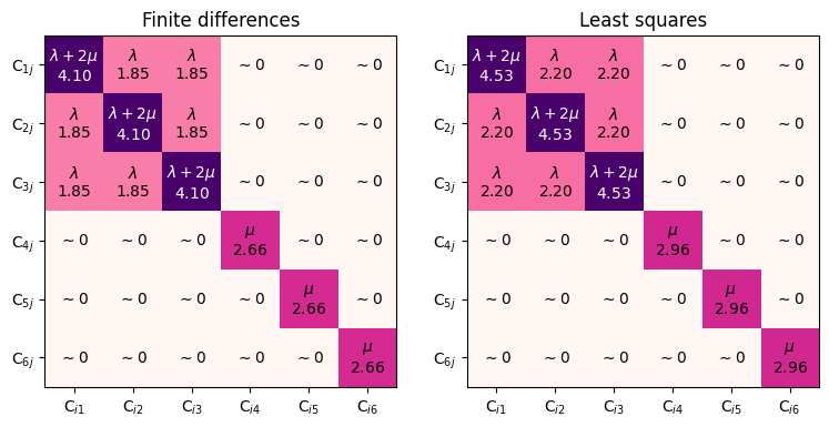
Let us first compute elastic constants with the matscipy.elasticity module, with two different functions:

measure_triclinic_elastic_constants computes the full Hooke’s tensor by finite differences
fit_elastic_constants computes a range of deformed configurations and fits a Hooke’s tensor with least-squares

from matscipy.elasticity import measure_triclinic_elastic_constants, fit_elastic_constants
from matscipy.elasticity import full_3x3x3x3_to_Voigt_6x6

C_finite_differences = full_3x3x3x3_to_Voigt_6x6(measure_triclinic_elastic_constants(system))
C_least_squares, _ = fit_elastic_constants(system, verbose=False)

Let’s plot the Hooke tensor:

import matplotlib.pyplot as plt

def spy_constants(ax, constants):
    ax.imshow(constants, cmap='RdPu', interpolation='none')
    labels = np.full_like(constants, "", dtype=object)
    labels[:3, :3] = "$\\lambda$\n"
    labels[(np.arange(3), np.arange(3))] = "$\\lambda + 2\\mu$\n"
    labels[(np.arange(3, 6), np.arange(3, 6))] = "$\\mu$\n"

    max_C = constants.max()
    
    for i in range(constants.shape[0]):
        for j in range(constants.shape[1]):
            color = "white" if constants[i, j] / max_C > 0.7 else "black"
            numeric = f"${constants[i, j]:.2f}$" if np.abs(constants[i, j]) / max_C > 1e-3 else "$\\sim 0$"

            ax.annotate(labels[i, j] + numeric,
                        (i, j),
                        horizontalalignment='center',
                        verticalalignment='center', color=color)
    
    ax.set_xticks(np.arange(constants.shape[1]))
    ax.set_yticks(np.arange(constants.shape[0]))
    ax.set_xticklabels([f"C$_{{i{j+1}}}$" for j in range(constants.shape[1])])
    ax.set_yticklabels([f"C$_{{{i+1}j}}$" for i in range(constants.shape[0])])

fig, axs = plt.subplots(1, 2, figsize=(9, 5))

spy_constants(axs[0], C_finite_differences)
spy_constants(axs[1], C_least_squares)

axs[0].set_title(f"Finite differences")
axs[1].set_title(f"Least squares")

plt.show()

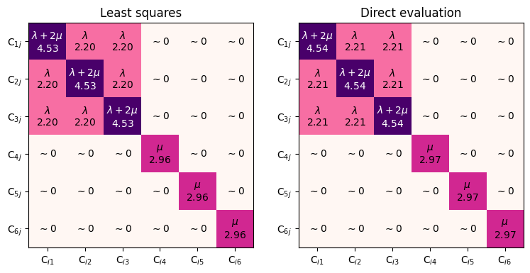
../_images/ca59943529ca39e786edcd46807910b8e09dfba4e43a9fbc960c2bd8404468b8.png

With second-order derivatives

Most calculators in matscipy actually implement second-order derivatives, and can therefore directly compute elastic constants:

C = full_3x3x3x3_to_Voigt_6x6(system.calc.get_property("elastic_constants", system))

fig, axs = plt.subplots(1, 2, figsize=(9, 5))

spy_constants(axs[0], C_least_squares)
spy_constants(axs[1], C)

axs[0].set_title(f"Least squares")
axs[1].set_title(f"Direct evaluation")

plt.show()

../_images/03cb7b91f6104e4bc0660bcaa1e00f74179018a58256f3502afbef07f1de2b06.png

Amorphous elastic constants

In amorphous solids, non-affine relaxation modes play an important role in elastic deformation.

Problem setup

Let’s randomize our atoms to mimic a glassy structure:

from ase.io import read
from pathlib import Path

data_path = Path("..") / ".." / "tests"

system = read(data_path / "CuZr_glass_460_atoms.gz")
interactive_view(system)

Setting up the calculator:

from matscipy.calculators.eam import EAM

system.calc = EAM(data_path / 'ZrCu.onecolumn.eam.alloy')

display(Latex(f"$E_\\mathrm{{pot}} = {system.get_potential_energy():.1f}$"))

\[E_\mathrm{pot} = -2244.3\]

Fitting elastic constants

The fit_elastic_constants function accepts a minimizer procedure as argument to account for non-affine relaxation modes.

from ase.optimize import FIRE

delta = 1e-4  # Configuration change increment

C_affine, _ = fit_elastic_constants(system, verbose=False, delta=delta)
C_relaxed, _ = fit_elastic_constants(system, verbose=False, delta=delta,
                                     # adjust fmax to desired precision
                                     optimizer=FIRE, fmax=5 * delta)

fig, axs = plt.subplots(1, 2, figsize=(9, 5))

spy_constants(axs[0], C_affine)
spy_constants(axs[1], C_relaxed)

axs[0].set_title(f"Affine only")
axs[1].set_title(f"Affine + Non-affine")

plt.show()

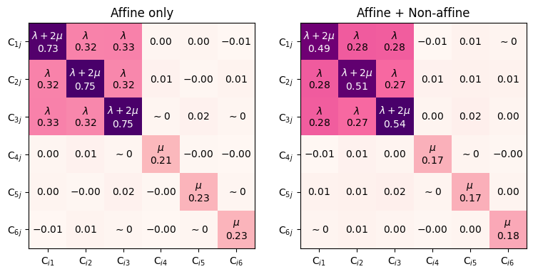
../_images/468f64f7afa7f48dfbb87a71dffda43cf71c6767d746752950c820e9bc1b78d8.png

One can see that elastic constants are significantly reduced when the internal relaxation is included. However, mind that the reduction is very dependent on the optimizer’s stopping criterion fmax, which should ideally be lower than the deformation increment (we set it higher in the example above for demonstration purposes only).