Pair-distribution function
The pair-distribution function describes the probability of finding a pair of atoms with a specific distance. We here describe how to compute a pair-distribution function \(g_2(r)\) of the type
where \(V\) is the overall volume of the simulation cell and \(N\) the total number of atoms (and hence \(N/V\) is the number density of the system). The average \(\langle\cdot\rangle\) is an ensemble average. This pair-distribution function has the property \(g_2(r)=1\) for \(r\to\infty\).
Real-space
The pair-distribution function above can be straightforwardly calculated from a neighbor list. We need to instruct the neighbor list to return the distance between atoms.
%matplotlib inline
import numpy as np
import matplotlib.pyplot as plt
from ase.io import read
from matscipy.neighbours import neighbour_list
# Load a disordered configuration (amorphous carbon)
a = read('../../tests/aC.cfg')
# Get distance between atoms up to a distance of 5 Angstroms
d = neighbour_list('d', a, cutoff=10.0)
# Get distance distribution - we broaden the delta-function into finite sized shells
n, x = np.histogram(d, bins=100, density=False)
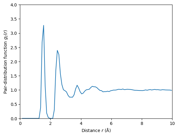
# Plot the pair-distribution function
mean_distance = (x[1:] + x[:-1])/2
mean_density = len(a) / a.get_volume()
shell_volume = 4 * np.pi * (x[1:] ** 3 - x[:-1] ** 3) / 3
plt.plot(mean_distance, n / (shell_volume * len(a) * mean_density))
plt.xlabel('Distance $r$ (Å)')
plt.ylabel('Pair-distribution function $g_2(r)$')
plt.xlim(0, 10)
plt.ylim(0, 4)
(0.0, 4.0)
Fourier space
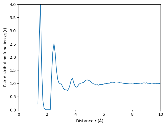
matscipy has utility function to compute pair-distribution (and other pair-correlation) functions. The utility function uses FFT to compute the long tail of the correlation function.
from matscipy.spatial_correlation_function import spatial_correlation_function

n, x = spatial_correlation_function(a, [1]*len(a), approx_FFT_gridsize=0.1)

plt.plot(x[x<10][1:], n[x<10][1:])
plt.xlabel('Distance $r$ (Å)')
plt.ylabel('Pair-distribution function $g_2(r)$')
plt.xlim(0, 10)
plt.ylim(0, 4)
(0.0, 4.0)