Molecular Dynamics Simulation of Fracture in Quartz
This tutorial has not been updated for the Python 3 rewrite of quippy. It is hosted here for archival purposes
This tutorial was prepared for use at a hands-on session at the Advanced Oxide Interfaces Workshop, ICTP, Trieste, May 2011.
Setting up your working environment
In this tutorial we are going to be using the QUIP (short for QUantum mechanics and Interatomic Potentials) code, which is a molecular dynamics code written in Fortran 95 and equipped with a Python interface named quippy.
As well as working with the standard unix command line we’ll also be using ipython, an interactive Python shell. In the listings below, shell commands are prefixed by a $ to identify them; everything else is a Python command which should be typed into the ipython shell. If you’re not familiar with Python don’t worry, it’s quite easy to pickup and the syntax is very similar to Fortran.
This tutorial assumes you have installed QUIP and quippy; see the Installation of QUIP and quippy section if you need some help on doing this.
Starting a fracture simulation
To maximise the amount of progress that we can make in the hands-on session, the first task is to get a fracture simulation running.
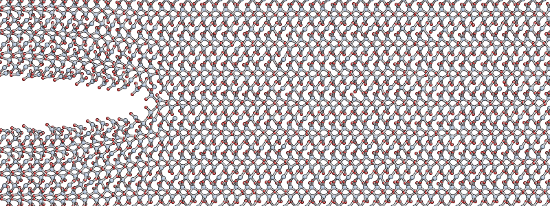
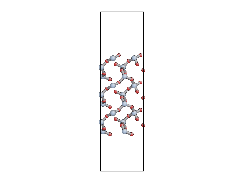
We’re going to be modelling a crack in \(\alpha\)-quartz opening
on the basal plane \((0001)\), with the crack front parallel to
the \([\bar{1}10]\) direction. The input structure is an
XYZ file contains a \(150~\AA
\times 50 \AA\) crack system with around 4000 atoms. The y axis is
aligned with the \((0001)\) plane, and the z axis with the
\([\bar{1}10]\) direction. The system contains a seed crack under
uniaxial tension in the y direction with a strain of 23%.
Download the following input files:
quartz_crack.xyz- the input structure, pictured above
quartz_crack.xml- parameters for potential and molecular dynamics
quartz_crack_bulk.xyz- structure of the quartz primitive cell
Before we begin, we need to make sure that the QUIP crack program is compiled by running the following commands:
$ export QUIP_ARCH=linux_x86_64_gfortran # or whichever arch is relevant
$ cd $QUIP_ROOT
$ make Programs/crack
Then press enter to accept default settings.
Note
The value you should assign to the variable QUIP_ARCH depends on your
platform (see Installation of QUIP and quippy for more details). QUIP_ROOT
refers to the directory where the the QUIP source code is located.
To make the command crack availale, copy the executable
${QUIP_ROOT}/build/${QUIP_ARCH} to a directory on your PATH,
e.g. ~/bin.
Similarly, to compile eval run:
$ make QUIP_Programs/eval
It is highly recommended to change the name when copying the eval prgram to a
directory on PATH to avoid a clash with the builtin eval command.
Start the simulation by running the crack program, which takes the “stem” of the input filenames as its only argument:
$ crack quartz_crack > quartz_crack.out &
Note that we’re redirecting the output to quartz_crack.out and running crack in the background. As well as outputting status information to quartz_crack.out, the simulation will periodically write the MD trajectory to a file named quartz_crack_movie_1.xyz.
You can monitor the progress of the simulation by opening the trajectory file with my modified version of AtomEye:
$ A quartz_crack_movie_1.xyz
In AtomEye, you can move the system within the periodic boundaries to centre it in the middle of the cell by holding Shift and dragging with your left mouse button, or by pressing Shift+z. Zoom in and out by dragging with the right mouse button. Press b to toggle the display of bonds. You can use the Insert and Delete keys to move forwards or backwards through the trajectory - note the frame number in the title bar of the window. You can quit AtomEye by pressing q.
For more help on AtomEye see its web page or my notes on this
modified version. In
particular, you might find this startup file
useful (copy to ~/.A to use).
Have a look at the output in quartz_crack.out. To see how the simulation is progressing, you can search this for lines starting with “D”:
$ grep "^D " quartz_crack.out
The first number gives the time in femtoseconds (the integration timestep of 0.5 fs is chosen to accurately sample the highest frequency phonon mode in the system), and the second and third are the instantaneous and time-averaged temperatures in Kelvin. The average temperature is computed using an exponential moving average.
After a few hundred femtoseconds, you should see the crack start to propagate in a fairly steady way, similar to the snapshot shown below (as a rough guide you can expect the simulation to progress at a rate of about 2 picoseconds per hour).
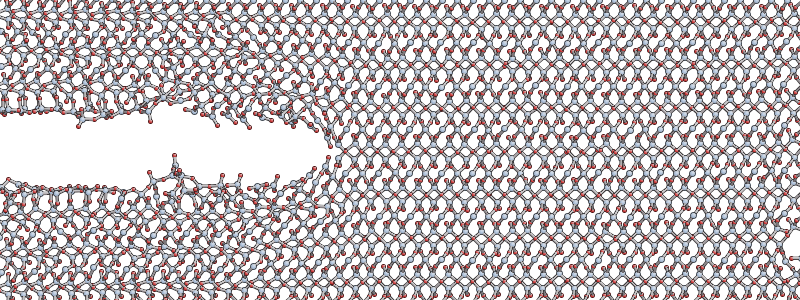
The simulation is run in the NVT ensemble, where the number of atoms N, volume V and temperature T are kept constant. The system is relatively small so a thermostat is used to regulate the temperature. The accelerating crack gives out a lot of energy, and since the thermostat used here is relatively weak, to avoid unduly influencing the dynamics, the temperature will initially rise before settling down once the crack reaches its equilbirum velocity.
Keep your crack simulation running as you proceed with the next parts of the tutorial (avoid closing the terminal in which you started the job!).
Quartz Primitive Unit Cell
While the fracture simulation is running, we will try to predict the expected behaviour of a crack in quartz according to continuum elasticity. We’ll start by performing some calculations on the quartz primitive cell using quippy.
Start ipython and import all the quippy routines:
$ ipython
...
In [1]: from quippy import *
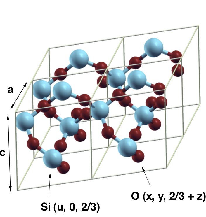
Construct an \(\alpha\)-quartz primitive unit cell and save it to an XYZ file:
aq = alpha_quartz(a=4.84038097073, c=5.3285240037, u=0.464175616171,
  x=0.411742710542, y=0.278727453998, z=0.109736032769)
aq.write("quartz.xyz")
Here a and c are the lattice parameters (in \(\AA\)), u is the internal displacement of the silicon atoms and x, y, and z the internal coordinates of the oxygens (see image below).
The variable aq is referred to as Atoms object. It contains
various attributes representing the system of interest which you can
inspect from the ipython command line, e.g. to print out the lattice
vectors, which are stored as columns in the lattice matrix
print aq.lattice
Or to print the atomic number and position of the first atom
print aq.z[1], aq.pos[1]
If you want to find out the syntax for a quippy function, type its name following by a question mark, e.g.
alpha_quartz ?
will print out the function signature and list of parameter types, as
well as a brief description of what alpha_quartz() does. If
you are interested in learning more about using QUIP and quippy,
you could take a look at the online tutorial-intro.
Keep your ipython session open as we’ll need it later. Open the quartz.xyz file you created with AtomEye. You should see something like this:
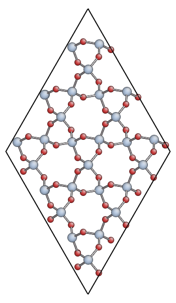
You can also download quartz.xyz for comparison.
Note
The main advantage of AtomEye is that it scales well to very larger systems, and does a pretty good job of understanding periodic boundary conditions. However, it can be a bit confusing for small cells like this. Since the quartz primitive cell contains only 9 atoms, AtomEye doubles the unit cell along the short lattice vectors (a and b) resulting in 36 atoms.
Calculating Elastic Properties
In order to predict the onset and velocity of fracture, we need to determine the values of the Young’s modulus \(E\), the Poisson ratio \(\nu\), surface energy density \(\gamma\) and the Rayleigh Wave speed \(c_R\). These are all properties of the classical potential which in this case is a short-ranged version of the TS polarisable potential (see this paper in J. Chem. Phys. for more about this potential).
Apart from \(\gamma\), all of these quantities can be obtained from the \(6 \times 6\) matrix of elastic constants \(C_{ij}\), so we will start by calculating this.
\(C\) is defined by \(\bm\sigma = C\bm\epsilon\) where \(\bm\sigma\) and \(\bm\epsilon\) are six component stress and strain vectors following the Voigt convention:
The simplest way to calculate \(C\) with QUIP is to use the
command line QUIP eval program. You will need the file quartz.xyz
you made earlier, as well as an XML file
containing the parameters of the classical potential:
$ eval init_args="IP TS" at_file=quartz.xyz param_file=TS_params.xml cij
Here init_args describes the kind of potential to use, at_file is the file containing the unit cell and param_file is the potential parameters. cij tells the eval program that we want it to calculate the elastic constants; this is done using the virial stress tensor. Have a look inside TS_params.xml to see the values which give the potential parameters controlling short range repsulsion, Yukawa-screened Coulomb interaction and dipole polarisability. For example you can see that oxygen (atomic number 8) is polarisable in this model and silicon (atomic number 14) is not.
Make a file called cij.dat containing the matrix output by eval (remove the “CIJ” at the beginning of each line). You can load this matrix into quippy using the command
C = loadtxt("cij.dat")
Extension: For trigonal crystals like \(\alpha\)-quartz, there are only actually 6 independent values in the \(C\) matrix:
where \(C_{66}\) is given by \(\frac{1}{2}(C_{11} - C_{12})\). We can exploit this symmetry to get all these values using only two strain patterns: \(\epsilon_{xx}\) and \(\epsilon_{yy}+\epsilon_{zz}\).
If you like, you could try using the following quippy code to evaluate \(C\) taking the cystal symmetry into account to see how the results differ from those obtained with eval.
p = Potential('IP TS', param_filename='TS_params.xml')
C = elastic_constants(p, aq, graphics=False, sym='trigonal_low')
Which components are most different? Why do you think this is? Think about the effect of internal relaxation: compare with the values of the \(C^0_{ij}\) tensor obtained if internal relaxation is not allowed (use the c0ij option to the eval program). Why do you think some components are particularily sensitive to internal relaxation?
Young’s Modulus and Poisson Ratio
To calculate the effective Young’s modulus and Poisson ratio for our quartz fracture simulation, we need to rotate the elastic constant matrix to align it with the axes of our \((0001)[\bar{1}10]\) fracture geometry. You can create the required rotation matrix using:
R = rotation_matrix(aq, (0,0,0,1), (-1,1,0))
print R
Next we transform \(C\) using the rotation matrix, and calculate the compliance matrix \(S = C^{-1}\):
C_eff = transform_elasticity(C, R)
S_eff = numpy.linalg.inv(C_eff)
C transforms as a rank-4 tensor since the full relation between stress and strain is \(\sigma_{ij} = c_{ijkl} \epsilon_{kl}\), meaning that the transformed tensor is
Finally we can work out the values of the effective Young’s modulus and Poisson ratio in the standard way from the components of the compliance matrix:
E = 1/S_eff[2,2]
print "Young's modulus", E, "GPa"

nu = -S_eff[1,2]/S_eff[2,2]
print "Poisson ratio", nu
Extension: Try rotating the quartz primitive cell directly:
aqr = transform(aq, R)
aqr.write("quartz_rotated.xyz")
Open quartz_rotated.xyz in AtomEye and confirm that it is oriented so that the \((0001)\) surface is aligned with the vertical (y) axis like the fracture system or quartz_0001.xyz, pictured below. Use eval to directly compute the elastic constant matrix of the rotated cell. How well does this matrix compare to C_eff?
Surface Energy
The file quartz_0001.xyz contains a 54 atom unit cell for
the (0001) surface of \(\alpha\)-quartz (shown below). Use either
the QUIP eval program or quippy to calculate the surface energy
density \(\gamma\) predicted by our classical potential for this
surface.
If you use eval, use the E command line option to get the program
to calculate the potential energy of the input cell. If you use
quippy, you should construct a Potential object using the
XML parameters from the file TS_params.xml as shown above. You can
then calculate the energy using the calc()
function - see the tutorial section on moleculardynamics for
more details.
Note
The energy unit of QUIP are electron volt (eV), and the distance units are Angstrom (\(\AA\)).
Hint: you can use the expression
where \(E_{surf}\) and \(E_{bulk}\) are the energies of surface and bulk configurations containing the same number of atoms, and \(A\) is the area of the open surface (with a factor of two because there are two open surfaces in this unit cell).
You should get a value for \(\gamma\) of around 3.5 J/m2.
Extension: what effect does relaxing the atomic positions have on
the surface energy? (use the relax argument to the eval
program, or the minim() function in quippy). What
happens if you anneal the surface using the md program?
$ md pot_init_args="IP TS" params_in_file=TS_params.xml \
    atoms_in_file=quartz_0001.xyz dt=0.5 N_steps=1000
Which surface energy do you think is more relevant for predicting the onset of fracture, relaxed or unrelaxed?
Energy Release Rate for Static Fracture
According to continuum elasticity, the strain energy release rate of an advancing crack is defined by
where \(U_E\) is the total strain energy and \(c\) is the crack length. The well-known Griffith criteria uses an energy-balance argument to equate the critical value of \(G\) at which fracture can first occur to the energy required to create two new surfaces.
According to Griffith, we should expect crack propagation to become favourable for \(G > 2\gamma\), where \(\gamma\) is the surface energy density.
Calculating G for a thin strip
We are using the thin strip geometry illustrated below for our fracture simulations, with the top and bottom edges fixed.
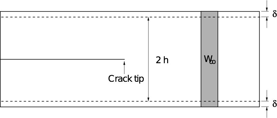
The advantage of this setup is that the energy release rate G does not depend on the crack length, and can be found analytically by considering the energetics of an advancing crack.
The horizontal edges of the strip are given a uniform normal displacement \(\delta\), so the applied strain is \(\epsilon_0 = \delta / h\). Far ahead of the crack, the strip is in uniaxial tension: \(\epsilon_{yy} \to \epsilon_0\) as \(x \to \infty\).
The stress far ahead of the crack is given by \(\sigma_{0} = E' \epsilon_{0}\), and therefore the elastic energy per unit length and per unit thickness far ahead of the crack tip is
where \(E'\) is the effective Young’s modulus.
Far behind the tip, the energy density is zero. Since no energy disappears through the clamped edges, if the crack is to advance by unit distance, a vertical strip of material with energy density \(W_\infty\) is effectively replaced by a strip with energy density zero.
The energy supplied to the crack tip is therefore equal to \(W_\infty\), so the energy release rate is simply
In our simulations we will use periodic boundary conditions in the \(z\) direction, so we have plane strain loading (\(\epsilon_{zz} = 0\)), which means that the effective Young’s modulus \(E'\) is given by \(E/(1-\nu^2)\), where \(E\) is the Young’s modulus in the \(y\) relevant direction and \(\nu\) is the Poisson ratio, so finally we have
Use your values for the Young’s modulus, Poisson ratio and surface energy to calculate the value of \(G\) (in units of J/m2) and strain \(\epsilon\) at which a sample of \(\alpha\)-quartz with a height of 50 \(\AA\) is expected to fracture according to the continuum Griffith criterium. How does this compare to the initial strain we applied to our fracture specimen?
Changing the loading of the fracture system
Once your crack simulation should has run for a couple of picoseconds the crack should have reached its terminal velocity so you can stop the simulation (you can do this nicely creating an empty file named stop_run, or simply by killing the process).
We are going to take the current state of the simulation and rescale it homogeneously to change the applied load. We will then continue the simulation starting from the rescaled system. In this way we will be able to investigate the relationship between the loading G and the equilibrium crack velocity V.
You should find a file named quartz_crack_check.xyz in your job directory. This is a checkpoint file which contains a full snapshot of all the instantaneous positions and velocities of the atoms in the system. Load this file into quippy and rescale it as follows:
a = Atoms('quartz_crack_check.xyz')
params = CrackParams('quartz_crack.xml')

b = crack_rescale_homogeneous_xy(a, params, new_strain)
b.write('quartz_crack_rescaled.xyz')
Replace new_strain with the target strain which should be between 0.15 and 0.30. If you inspect the new file quartz_crack_rescaled.xyz you should see it’s identical to the orignal apart from the rescaling in the x and y directions (not along z since the system is periodic in that direction). Copy the bulk cell and XML parameters and start a new crack simulation:
$ cp quartz_crack_bulk.xyz quartz_crack_rescaled_bulk.xyz
$ cp quartz_crack.xml quartz_crack_rescaled.xml
$ crack quartz_crack_rescaled > quartz_crack_rescaled.out &
Wait for the restarted simulation to reach a steady state and then
estimate the crack velocity from looking at the XYZ file (right-click
on an atom in AtomEye to print out its position; the interval
between frames is 10 fs) or by plotting the crack position as a
function of time by extracting lines starting with CRACK_TIP from
the output file (you might find this crack-velo.sh script
useful to do this; note however that the crack tip position is found
using the atomic coordination numbers so if thre are defects in your
cell it will not work correctly).
Energy Release Rate for Dynamic Fracture
Freund extended this approach to dynamic fracture by writing the total energy required to break bonds at the crack surface as the product of the static energy release rate \(G\) and a universal velocity-dependent function which he showed can be approximated as a linear function of the crack speed \(V\)
The Rayleigh surface wave speed \(c_R\) sets the ultimate limit for the crack propagation speed. The expected velocity as a function of the loading \(G/2\gamma\) is then
This is the Freund equation of motion. Calculating the Rayleigh wave speed - the speed with which elastic waves travel on a free surface - is fairly straightforward for isotropic materials. For anisotropic materials like quartz the calculation is more involved since the speed will be different for wave propagation in different crystallographic directions. For our case, the value turns out to be \(c_R \sim 9.3\) km/s using the elastic constants calculated for the short-range TS classical potential.
How does your measured value for the crack velocity compare to that predicted by the Freund equation of motion for the same G?
At the end of the session we will try to combine everybody’s results to produce a plot of \(V(G)\).
Extension tasks
Look carefully at the MD trajectory from your fracture simulation in AtomEye. Do you notice anything about the bond-breaking events at the crack tip? How would you calculate the amount of charge which ends up on each of the cleaved surfaces?
What is the effect of changing the simulation temperature? Trying changing the value of sim_temp in the XML parameter file to something much larger, e.g. 1000 K. Is the fracture qualitatively different? What happens if you turn off the thermostat (change the ensemble setting from NVT to NVE).
The expression \(E_y = 1/S_{22}\) is an approximation and is not strictly valid for hexagonal materials. Check this approximation by performing a tensile test: take the rotated configuration aqr apply a series of small strains in the y direction, and compute the stress using the classical potential, using code based on the following:
p = Potential('IP TS', param_filename='TS_params.xml')
...
T = numpy.diag([1., 1+.eps_yy, 1.])            # matrix for strain in y
aqr_t = transform(aqr, T)                      # apply transformation
p.calc(aqr_t, virial=True)                     # compute virial tensor
sig_yy = -v[2,2]/aqr_t.cell_volume()*GPA       # convert to stress
Calculate an improved estimate for \(E_y\) by fitting a straight line to sig_yy as function of eps_yy. How good is the approximation we used above?
It’s important to bear in mind that what we’ve done here is necessarily very approximate for a number of reasons:
This is a very small system
The applied loading is very large
The description of bond-breaking provided by classical potential is simplistic
Which of these do you think is most important? How could these limitations be overcome in a more complete simulation?
Input files and Solutions
quartz_crack.xyz,quartz_crack.xml,quartz_crack_bulk.xyz- input files for crack simulationquartz.xyz- quartz primitive cellquartz_0001.xyz- quartz (0001) surface cellTS_params.xml- potential parameterselastic.sh- script to compute elastic constantscij.dat- elastic constants obtained with eval programsurface-energy.sh- script to compute surface energysurface-energy-relaxed.sh- script to compute relaxed surface energysurface-energy-annealed.sh- script to compute annealed surface energycrack-velo.sh- script to crack velocity