How to train a GAP model from scratch
steps
1. generate a small dataset of water structures
    - use CP2K if you have access to it
    - otherwise: use any simple potential implemented in ASE, just for trying this out I have used EMT here
1. generate e0 values: isolated atoms in the dataset
1. separate a training and a validation dataset
1. **train the model**
1. look at the outcome of the model
here we will fit twice, to see the difference between a 2b-only and a 2b+3b fit
[15]:
# general imports
import numpy as np
import matplotlib.pyplot as plt
from copy import deepcopy as cp

# ase imports
import ase.io
from ase import Atoms, Atom
from ase import units
from ase.build import molecule
# for MD
from ase.md.langevin import Langevin
from ase.io.trajectory import Trajectory
[2]:
# helper functions
def make_water(density, super_cell=[3, 3, 3]):
    """ Geenrates a supercell of water molecules with a desired density.
        Density in g/cm^3!!!"""
    h2o = molecule('H2O')
    a = np.cbrt((sum(h2o.get_masses()) * units.m ** 3 * 1E-6 ) / (density * units.mol))
    h2o.set_cell((a, a, a))
    h2o.set_pbc((True, True, True))
    #return cp(h2o.repeat(super_cell))
    return h2o.repeat(super_cell)

def rms_dict(x_ref, x_pred):
    """ Takes two datasets of the same shape and returns a dictionary containing RMS error data"""

    x_ref = np.array(x_ref)
    x_pred = np.array(x_pred)

    if np.shape(x_pred) != np.shape(x_ref):
        raise ValueError('WARNING: not matching shapes in rms')

    error_2 = (x_ref - x_pred) ** 2

    average = np.sqrt(np.average(error_2))
    std_ = np.sqrt(np.var(error_2))

    return {'rmse': average, 'std': std_}
generating data only with ASE, using the EMT calculator
This is only for the demonstration of how to do it, this run is will be done very fast. There is no practical use of the data beyond learning the use teach_sparse, quip, etc. with it.
[3]:
# Running MD with ASE's EMT

from ase.calculators.emt import EMT
calc = EMT()

T = 150  # Kelvin

# Set up a grid of water
water = make_water(1.0, [3, 3, 3])
water.set_calculator(calc)

# We want to run MD using the Langevin algorithm
# with a time step of 1 fs, the temperature T and the friction
# coefficient to 0.002 atomic units.
dyn = Langevin(water, 1 * units.fs, T * units.kB, 0.0002)

def printenergy(a=water):  # store a reference to atoms in the definition.
    """Function to print the potential, kinetic and total energy."""
    epot = a.get_potential_energy() / len(a)
    ekin = a.get_kinetic_energy() / len(a)
    print('Energy per atom: Epot = %.3feV  Ekin = %.3feV (T=%3.0fK)  '
          'Etot = %.3feV' % (epot, ekin, ekin / (1.5 * units.kB), epot + ekin))

dyn.attach(printenergy, interval=5)

# We also want to save the positions of all atoms after every 5th time step.
traj = Trajectory('dyn_emt.traj', 'w', water)
dyn.attach(traj.write, interval=5)

# Now run the dynamics
printenergy(water)
dyn.run(600)   # CHANGE THIS IF YOU WANT LONGER/SHORTER RUN
Energy per atom: Epot = 0.885eV  Ekin = 0.000eV (T=  0K)  Etot = 0.885eV
Energy per atom: Epot = 0.820eV  Ekin = 0.053eV (T=413K)  Etot = 0.874eV
Energy per atom: Epot = 0.660eV  Ekin = 0.208eV (T=1611K)  Etot = 0.868eV
Energy per atom: Epot = 0.632eV  Ekin = 0.224eV (T=1736K)  Etot = 0.857eV
Energy per atom: Epot = 0.869eV  Ekin = 0.005eV (T= 39K)  Etot = 0.874eV
Energy per atom: Epot = 0.781eV  Ekin = 0.088eV (T=682K)  Etot = 0.869eV
Energy per atom: Epot = 0.756eV  Ekin = 0.117eV (T=903K)  Etot = 0.872eV
Energy per atom: Epot = 0.706eV  Ekin = 0.164eV (T=1270K)  Etot = 0.870eV
Energy per atom: Epot = 0.703eV  Ekin = 0.158eV (T=1223K)  Etot = 0.861eV
Energy per atom: Epot = 0.867eV  Ekin = 0.006eV (T= 47K)  Etot = 0.873eV
Energy per atom: Epot = 0.704eV  Ekin = 0.160eV (T=1241K)  Etot = 0.864eV
Energy per atom: Epot = 0.679eV  Ekin = 0.190eV (T=1468K)  Etot = 0.868eV
Energy per atom: Epot = 0.822eV  Ekin = 0.051eV (T=391K)  Etot = 0.872eV
Energy per atom: Epot = 0.782eV  Ekin = 0.088eV (T=677K)  Etot = 0.869eV
Energy per atom: Epot = 0.775eV  Ekin = 0.096eV (T=739K)  Etot = 0.871eV
Energy per atom: Epot = 0.751eV  Ekin = 0.119eV (T=920K)  Etot = 0.870eV
Energy per atom: Epot = 0.752eV  Ekin = 0.117eV (T=904K)  Etot = 0.869eV
Energy per atom: Epot = 0.764eV  Ekin = 0.107eV (T=825K)  Etot = 0.871eV
Energy per atom: Epot = 0.752eV  Ekin = 0.120eV (T=927K)  Etot = 0.871eV
Energy per atom: Epot = 0.747eV  Ekin = 0.123eV (T=953K)  Etot = 0.871eV
Energy per atom: Epot = 0.724eV  Ekin = 0.145eV (T=1119K)  Etot = 0.868eV
Energy per atom: Epot = 0.703eV  Ekin = 0.166eV (T=1281K)  Etot = 0.869eV
Energy per atom: Epot = 0.738eV  Ekin = 0.132eV (T=1022K)  Etot = 0.870eV
Energy per atom: Epot = 0.703eV  Ekin = 0.165eV (T=1280K)  Etot = 0.868eV
Energy per atom: Epot = 0.697eV  Ekin = 0.172eV (T=1331K)  Etot = 0.869eV
Energy per atom: Epot = 0.731eV  Ekin = 0.140eV (T=1083K)  Etot = 0.871eV
Energy per atom: Epot = 0.716eV  Ekin = 0.155eV (T=1199K)  Etot = 0.871eV
Energy per atom: Epot = 0.706eV  Ekin = 0.163eV (T=1257K)  Etot = 0.869eV
Energy per atom: Epot = 0.721eV  Ekin = 0.149eV (T=1151K)  Etot = 0.870eV
Energy per atom: Epot = 0.685eV  Ekin = 0.184eV (T=1424K)  Etot = 0.869eV
Energy per atom: Epot = 0.706eV  Ekin = 0.164eV (T=1271K)  Etot = 0.870eV
Energy per atom: Epot = 0.721eV  Ekin = 0.150eV (T=1161K)  Etot = 0.871eV
Energy per atom: Epot = 0.690eV  Ekin = 0.180eV (T=1396K)  Etot = 0.870eV
Energy per atom: Epot = 0.663eV  Ekin = 0.207eV (T=1601K)  Etot = 0.870eV
Energy per atom: Epot = 0.623eV  Ekin = 0.247eV (T=1907K)  Etot = 0.869eV
Energy per atom: Epot = 0.609eV  Ekin = 0.261eV (T=2022K)  Etot = 0.870eV
Energy per atom: Epot = 0.576eV  Ekin = 0.294eV (T=2271K)  Etot = 0.870eV
Energy per atom: Epot = 0.563eV  Ekin = 0.306eV (T=2370K)  Etot = 0.870eV
Energy per atom: Epot = 0.571eV  Ekin = 0.298eV (T=2307K)  Etot = 0.869eV
Energy per atom: Epot = 0.605eV  Ekin = 0.265eV (T=2050K)  Etot = 0.870eV
Energy per atom: Epot = 0.566eV  Ekin = 0.302eV (T=2338K)  Etot = 0.869eV
Energy per atom: Epot = 0.579eV  Ekin = 0.290eV (T=2242K)  Etot = 0.868eV
Energy per atom: Epot = 0.580eV  Ekin = 0.289eV (T=2234K)  Etot = 0.868eV
Energy per atom: Epot = 0.557eV  Ekin = 0.311eV (T=2406K)  Etot = 0.868eV
Energy per atom: Epot = 0.605eV  Ekin = 0.264eV (T=2046K)  Etot = 0.870eV
Energy per atom: Epot = 0.541eV  Ekin = 0.327eV (T=2530K)  Etot = 0.868eV
Energy per atom: Epot = 0.521eV  Ekin = 0.347eV (T=2686K)  Etot = 0.868eV
Energy per atom: Epot = 0.535eV  Ekin = 0.339eV (T=2622K)  Etot = 0.874eV
Energy per atom: Epot = 0.540eV  Ekin = 0.333eV (T=2574K)  Etot = 0.873eV
Energy per atom: Epot = 0.597eV  Ekin = 0.278eV (T=2151K)  Etot = 0.875eV
Energy per atom: Epot = 0.534eV  Ekin = 0.340eV (T=2631K)  Etot = 0.874eV
Energy per atom: Epot = 0.490eV  Ekin = 0.384eV (T=2968K)  Etot = 0.874eV
Energy per atom: Epot = 0.496eV  Ekin = 0.378eV (T=2928K)  Etot = 0.875eV
Energy per atom: Epot = 0.495eV  Ekin = 0.384eV (T=2970K)  Etot = 0.879eV
Energy per atom: Epot = 0.456eV  Ekin = 0.424eV (T=3277K)  Etot = 0.880eV
Energy per atom: Epot = 0.454eV  Ekin = 0.430eV (T=3325K)  Etot = 0.883eV
Energy per atom: Epot = 0.527eV  Ekin = 0.358eV (T=2767K)  Etot = 0.884eV
Energy per atom: Epot = 0.493eV  Ekin = 0.391eV (T=3027K)  Etot = 0.885eV
Energy per atom: Epot = 0.496eV  Ekin = 0.389eV (T=3011K)  Etot = 0.885eV
Energy per atom: Epot = 0.500eV  Ekin = 0.384eV (T=2971K)  Etot = 0.884eV
Energy per atom: Epot = 0.508eV  Ekin = 0.374eV (T=2895K)  Etot = 0.882eV
Energy per atom: Epot = 0.470eV  Ekin = 0.411eV (T=3176K)  Etot = 0.881eV
Energy per atom: Epot = 0.430eV  Ekin = 0.451eV (T=3489K)  Etot = 0.881eV
Energy per atom: Epot = 0.404eV  Ekin = 0.478eV (T=3696K)  Etot = 0.882eV
Energy per atom: Epot = 0.410eV  Ekin = 0.471eV (T=3645K)  Etot = 0.881eV
Energy per atom: Epot = 0.473eV  Ekin = 0.408eV (T=3160K)  Etot = 0.881eV
Energy per atom: Epot = 0.429eV  Ekin = 0.451eV (T=3490K)  Etot = 0.880eV
Energy per atom: Epot = 0.439eV  Ekin = 0.442eV (T=3423K)  Etot = 0.881eV
Energy per atom: Epot = 0.465eV  Ekin = 0.416eV (T=3216K)  Etot = 0.881eV
Energy per atom: Epot = 0.448eV  Ekin = 0.432eV (T=3346K)  Etot = 0.880eV
Energy per atom: Epot = 0.465eV  Ekin = 0.417eV (T=3222K)  Etot = 0.882eV
Energy per atom: Epot = 0.457eV  Ekin = 0.423eV (T=3274K)  Etot = 0.880eV
Energy per atom: Epot = 0.425eV  Ekin = 0.456eV (T=3528K)  Etot = 0.881eV
Energy per atom: Epot = 0.415eV  Ekin = 0.465eV (T=3598K)  Etot = 0.880eV
Energy per atom: Epot = 0.458eV  Ekin = 0.427eV (T=3301K)  Etot = 0.884eV
Energy per atom: Epot = 0.444eV  Ekin = 0.442eV (T=3423K)  Etot = 0.886eV
Energy per atom: Epot = 0.386eV  Ekin = 0.499eV (T=3858K)  Etot = 0.885eV
Energy per atom: Epot = 0.386eV  Ekin = 0.499eV (T=3864K)  Etot = 0.885eV
Energy per atom: Epot = 0.421eV  Ekin = 0.466eV (T=3609K)  Etot = 0.887eV
Energy per atom: Epot = 0.390eV  Ekin = 0.498eV (T=3854K)  Etot = 0.888eV
Energy per atom: Epot = 0.404eV  Ekin = 0.488eV (T=3777K)  Etot = 0.892eV
Energy per atom: Epot = 0.411eV  Ekin = 0.480eV (T=3714K)  Etot = 0.891eV
Energy per atom: Epot = 0.429eV  Ekin = 0.460eV (T=3558K)  Etot = 0.889eV
Energy per atom: Epot = 0.391eV  Ekin = 0.497eV (T=3848K)  Etot = 0.888eV
Energy per atom: Epot = 0.379eV  Ekin = 0.507eV (T=3924K)  Etot = 0.886eV
Energy per atom: Epot = 0.429eV  Ekin = 0.460eV (T=3555K)  Etot = 0.889eV
Energy per atom: Epot = 0.431eV  Ekin = 0.458eV (T=3545K)  Etot = 0.889eV
Energy per atom: Epot = 0.440eV  Ekin = 0.447eV (T=3458K)  Etot = 0.887eV
Energy per atom: Epot = 0.417eV  Ekin = 0.467eV (T=3610K)  Etot = 0.884eV
Energy per atom: Epot = 0.445eV  Ekin = 0.442eV (T=3422K)  Etot = 0.888eV
Energy per atom: Epot = 0.437eV  Ekin = 0.447eV (T=3461K)  Etot = 0.884eV
Energy per atom: Epot = 0.439eV  Ekin = 0.447eV (T=3460K)  Etot = 0.886eV
Energy per atom: Epot = 0.424eV  Ekin = 0.464eV (T=3587K)  Etot = 0.888eV
Energy per atom: Epot = 0.394eV  Ekin = 0.493eV (T=3817K)  Etot = 0.887eV
Energy per atom: Epot = 0.370eV  Ekin = 0.515eV (T=3984K)  Etot = 0.885eV
Energy per atom: Epot = 0.373eV  Ekin = 0.511eV (T=3951K)  Etot = 0.883eV
Energy per atom: Epot = 0.402eV  Ekin = 0.485eV (T=3748K)  Etot = 0.886eV
Energy per atom: Epot = 0.380eV  Ekin = 0.506eV (T=3912K)  Etot = 0.886eV
Energy per atom: Epot = 0.404eV  Ekin = 0.483eV (T=3736K)  Etot = 0.887eV
Energy per atom: Epot = 0.443eV  Ekin = 0.444eV (T=3436K)  Etot = 0.887eV
Energy per atom: Epot = 0.419eV  Ekin = 0.469eV (T=3626K)  Etot = 0.888eV
Energy per atom: Epot = 0.440eV  Ekin = 0.451eV (T=3489K)  Etot = 0.891eV
Energy per atom: Epot = 0.434eV  Ekin = 0.453eV (T=3505K)  Etot = 0.887eV
Energy per atom: Epot = 0.423eV  Ekin = 0.468eV (T=3619K)  Etot = 0.891eV
Energy per atom: Epot = 0.369eV  Ekin = 0.523eV (T=4047K)  Etot = 0.892eV
Energy per atom: Epot = 0.413eV  Ekin = 0.478eV (T=3701K)  Etot = 0.891eV
Energy per atom: Epot = 0.359eV  Ekin = 0.531eV (T=4108K)  Etot = 0.890eV
Energy per atom: Epot = 0.401eV  Ekin = 0.491eV (T=3799K)  Etot = 0.892eV
Energy per atom: Epot = 0.414eV  Ekin = 0.477eV (T=3688K)  Etot = 0.890eV
Energy per atom: Epot = 0.376eV  Ekin = 0.513eV (T=3969K)  Etot = 0.889eV
Energy per atom: Epot = 0.368eV  Ekin = 0.522eV (T=4035K)  Etot = 0.890eV
Energy per atom: Epot = 0.370eV  Ekin = 0.521eV (T=4029K)  Etot = 0.891eV
Energy per atom: Epot = 0.379eV  Ekin = 0.512eV (T=3959K)  Etot = 0.891eV
Energy per atom: Epot = 0.393eV  Ekin = 0.502eV (T=3881K)  Etot = 0.894eV
Energy per atom: Epot = 0.373eV  Ekin = 0.515eV (T=3984K)  Etot = 0.888eV
Energy per atom: Epot = 0.367eV  Ekin = 0.530eV (T=4100K)  Etot = 0.897eV
Energy per atom: Epot = 0.380eV  Ekin = 0.520eV (T=4026K)  Etot = 0.900eV
Energy per atom: Epot = 0.384eV  Ekin = 0.523eV (T=4048K)  Etot = 0.908eV
Energy per atom: Epot = 0.417eV  Ekin = 0.485eV (T=3751K)  Etot = 0.902eV
Energy per atom: Epot = 0.402eV  Ekin = 0.518eV (T=4005K)  Etot = 0.919eV
Energy per atom: Epot = 0.417eV  Ekin = 0.558eV (T=4313K)  Etot = 0.974eV
[4]:
# wrap and save traj in .xyz --- the .traj is a non human readable database file, xyz is much better
out_traj = ase.io.read('dyn_emt.traj', ':')
for at in out_traj:
    at.wrap()
    if 'momenta' in at.arrays: del at.arrays['momenta']
ase.io.write('dyn_emt.xyz', out_traj, 'xyz')
get e0 for H and O - energies of the isolated atoms
This is the energy of the isolated atom, will be in the teach_sparse string in the following format: e0={H:energy:O:energy}
[5]:
isolated_H = Atoms('H', calculator=EMT())
isolated_O = Atoms('O', calculator=EMT())

print('e0_H:',isolated_H.get_potential_energy())
print('e0_O:',isolated_O.get_potential_energy())

# this made the e0 string be the following: e0={H:3.21:O:4.6}
e0_H: 3.21
e0_O: 4.6
separate the dataset into a training and a validation set
As we have 120 frames from the 600fs MD, I will do it 60,60 with taking even and odd frames for the two
[6]:
ase.io.write('train.xyz', out_traj[0::2])
ase.io.write('validate.xyz', out_traj[1::2])
[7]:
out_traj[0].arrays.keys()
[7]:
dict_keys(['numbers', 'positions'])
train our GAP model from the command line
Will use a fit of 2b only, using the desciptor distance_2b.
Let’s understand how this works. The bash command takes named arguments separated by spaces.
teach_sparsethe command which actually does the fite0={H:3.21:O:4.6}the energies of the isolated atomsenergy_parameter_name=energy force_parameter_name=forcesnames of the parametersdo_copy_at_file=F sparse_separate_file=Tjust needed, don’t want to copy the training data and using separate files for the xml makes it fastergp_file=GAP.xmlfilename of the potential parameters, I have always used this name, because I had separate directories for the different trainings potentialsat_file=train.xyztraining filedefault_sigma={0.008 0.04 0 0}sigma values to be used for energies, forces, stresses, hessians in order; this represents the accuracy of the data and the relative weight of them in the fit (more accurate –> more significant in the fit)gap={...}the potential to be fit, separated by ‘:’
distance_2b - cutoff=4.0 radial, practically the highest distance the descriptor takes into account - covariance_type=ard_se use gausses in the fit - delta=0.5 what relative portion of the things shall be determined by this potential - theta_uniform=1.0 width of the gaussians - sparse_method=uniform use uniform bins to choose the sparse points - add_species=T take the species into account, so it will generate more GAPs automatically (see the output) - n_sparse=10
number of sparse points
notice, that the script is running in parallel, using all 8 cores of the current machine
[8]:
! teach_sparse e0={H:3.21:O:4.6} energy_parameter_name=energy force_parameter_name=forces do_copy_at_file=F sparse_separate_file=T gp_file=GAP.xml at_file=train.xyz default_sigma={0.008 0.04 0 0} gap={distance_2b cutoff=4.0 covariance_type=ard_se delta=0.5 theta_uniform=1.0 sparse_method=uniform add_species=T n_sparse=10}
libAtoms::Hello World: 07/10/2018   18:10:52
libAtoms::Hello World: git version  https://github.com/libAtoms/QUIP.git,531330f-dirty
libAtoms::Hello World: QUIP_ARCH    linux_x86_64_gfortran_openmp
libAtoms::Hello World: compiled on  Jul  2 2018 at 21:44:13
libAtoms::Hello World: OpenMP parallelisation with 8 threads
WARNING: libAtoms::Hello World: environment variable OMP_STACKSIZE not set explicitly. The default value - system and compiler dependent - may be too small for some applications.
libAtoms::Hello World: Random Seed = 65452599
libAtoms::Hello World: global verbosity = 0

Calls to system_timer will do nothing by default


================================ Input parameters ==============================

at_file = train.xyz
gap = "distance_2b cutoff=4.0 covariance_type=ard_se delta=0.5 theta_uniform=1.0 sparse_method=uniform add_species=T n_sparse=10"
e0 = H:3.21:O:4.6
e0_offset = 0.0
do_e0_avg = T
default_sigma = "0.008 0.04 0 0"
sparse_jitter = 1.0e-10
hessian_delta = 1.0e-2
core_param_file = quip_params.xml
core_ip_args =
energy_parameter_name = energy
force_parameter_name = forces
virial_parameter_name = virial
hessian_parameter_name = hessian
config_type_parameter_name = config_type
sigma_parameter_name = sigma
config_type_sigma =
sigma_per_atom = T
do_copy_at_file = F
sparse_separate_file = T
sparse_use_actual_gpcov = F
gp_file = GAP.xml
verbosity = NORMAL
rnd_seed = -1
do_ip_timing = F
template_file = template.xyz

========================================  ======================================


============== Gaussian Approximation Potentials - Database fitting ============


Initial parsing of command line arguments finished.
Found 1 GAPs.
Descriptors have been parsed
XYZ file read
Old GAP: {distance_2b cutoff=4.0 covariance_type=ard_se delta=0.5 theta_uniform=1.0 sparse_method=uniform add_species=T n_sparse=10}
New GAP: {distance_2b cutoff=4.0 covariance_type=ard_se delta=0.5 theta_uniform=1.0 sparse_method=uniform               n_sparse=10 Z1=8 Z2=8}
New GAP: {distance_2b cutoff=4.0 covariance_type=ard_se delta=0.5 theta_uniform=1.0 sparse_method=uniform               n_sparse=10 Z1=8 Z2=1}
New GAP: {distance_2b cutoff=4.0 covariance_type=ard_se delta=0.5 theta_uniform=1.0 sparse_method=uniform               n_sparse=10 Z1=1 Z2=1}
Multispecies support added where requested
Number of target energies (property name: energy) found: 60
Number of target forces (property name: forces) found: 14580
Number of target virials (property name: virial) found: 0
Number of target Hessian eigenvalues (property name: hessian) found: 0
Cartesian coordinates transformed to descriptors
Started sparse covariance matrix calculation of coordinate 1

Finished sparse covariance matrix calculation of coordinate 1
TIMER: gpFull_covarianceMatrix_sparse_Coordinate1_sparse  done in .91605700000000012 cpu secs, .11785597354173660 wall clock secs.
TIMER: gpFull_covarianceMatrix_sparse_Coordinate1         done in .91605700000000012 cpu secs, .11797238700091839 wall clock secs.
Started sparse covariance matrix calculation of coordinate 2

Finished sparse covariance matrix calculation of coordinate 2
TIMER: gpFull_covarianceMatrix_sparse_Coordinate2_sparse  done in 3.7722349999999998 cpu secs, .47368377633392811 wall clock secs.
TIMER: gpFull_covarianceMatrix_sparse_Coordinate2         done in 3.7722349999999998 cpu secs, .47379869595170021 wall clock secs.
Started sparse covariance matrix calculation of coordinate 3

Finished sparse covariance matrix calculation of coordinate 3
TIMER: gpFull_covarianceMatrix_sparse_Coordinate3_sparse  done in 3.5482220000000000 cpu secs, .44678380154073238 wall clock secs.
TIMER: gpFull_covarianceMatrix_sparse_Coordinate3         done in 3.5522219999999995 cpu secs, .44689681194722652 wall clock secs.
TIMER: gpFull_covarianceMatrix_sparse_LinearAlgebra       done in .56005000000000749E-001 cpu secs, .13479800894856453E-001 wall clock secs.
TIMER: gpFull_covarianceMatrix_sparse_FunctionValues      done in .00000000000000000E+000 cpu secs, .14016032218933105E-003 wall clock secs.
TIMER: gpFull_covarianceMatrix_sparse                     done in 8.3005189999999995 cpu secs, 1.0586479119956493 wall clock secs.
TIMER: GP sparsify                                        done in 9.8286140000000000 cpu secs, 1.4589964970946312 wall clock secs.

libAtoms::Finalise: 07/10/2018   18:10:55
libAtoms::Finalise: Bye-Bye!
use the potential with QUIP on trani.xyz and validate.xyz
[9]:
# calculate train.xyz

! quip E=T F=T atoms_filename=train.xyz param_filename=GAP.xml | grep AT | sed 's/AT//' >> quip_train.xyz
! quip E=T F=T atoms_filename=validate.xyz param_filename=GAP.xml | grep AT | sed 's/AT//' >> quip_validate.xyz
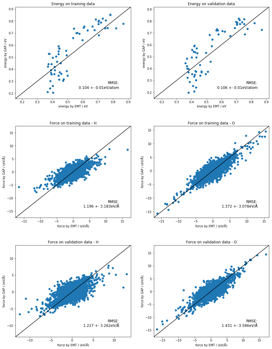
make simple plots of the energies and forces on the EMT and GAP datas
[16]:
def energy_plot(in_file, out_file, ax, title='Plot of energy'):
    """ Plots the distribution of energy per atom on the output vs the input"""
    # read files
    in_atoms = ase.io.read(in_file, ':')
    out_atoms = ase.io.read(out_file, ':')
    # list energies
    ener_in = [at.get_potential_energy() / len(at.get_chemical_symbols()) for at in in_atoms]
    ener_out = [at.get_potential_energy() / len(at.get_chemical_symbols()) for at in out_atoms]
    # scatter plot of the data
    ax.scatter(ener_in, ener_out)
    # get the appropriate limits for the plot
    for_limits = np.array(ener_in +ener_out)
    elim = (for_limits.min() - 0.05, for_limits.max() + 0.05)
    ax.set_xlim(elim)
    ax.set_ylim(elim)
    # add line of slope 1 for refrence
    ax.plot(elim, elim, c='k')
    # set labels
    ax.set_ylabel('energy by GAP / eV')
    ax.set_xlabel('energy by EMT / eV')
    #set title
    ax.set_title(title)
    # add text about RMSE
    _rms = rms_dict(ener_in, ener_out)
    rmse_text = 'RMSE:\n' + str(np.round(_rms['rmse'], 3)) + ' +- ' + str(np.round(_rms['std'], 3)) + 'eV/atom'
    ax.text(0.9, 0.1, rmse_text, transform=ax.transAxes, fontsize='large', horizontalalignment='right',
            verticalalignment='bottom')

def force_plot(in_file, out_file, ax, symbol='HO', title='Plot of force'):
    """ Plots the distribution of firce components per atom on the output vs the input
        only plots for the given atom type(s)"""

    in_atoms = ase.io.read(in_file, ':')
    out_atoms = ase.io.read(out_file, ':')

    # extract data for only one species
    in_force, out_force = [], []
    for at_in, at_out in zip(in_atoms, out_atoms):
        # get the symbols
        sym_all = at_in.get_chemical_symbols()
        # add force for each atom
        for j, sym in enumerate(sym_all):
            if sym in symbol:
                in_force.append(at_in.get_forces()[j])
                #out_force.append(at_out.get_forces()[j]) \
                out_force.append(at_out.arrays['force'][j]) # because QUIP and ASE use different names
    # convert to np arrays, much easier to work with
    #in_force = np.array(in_force)
    #out_force = np.array(out_force)
    # scatter plot of the data
    ax.scatter(in_force, out_force)
    # get the appropriate limits for the plot
    for_limits = np.array(in_force + out_force)
    flim = (for_limits.min() - 1, for_limits.max() + 1)
    ax.set_xlim(flim)
    ax.set_ylim(flim)
    # add line of
    ax.plot(flim, flim, c='k')
    # set labels
    ax.set_ylabel('force by GAP / (eV/Å)')
    ax.set_xlabel('force by EMT / (eV/Å)')
    #set title
    ax.set_title(title)
    # add text about RMSE
    _rms = rms_dict(in_force, out_force)
    rmse_text = 'RMSE:\n' + str(np.round(_rms['rmse'], 3)) + ' +- ' + str(np.round(_rms['std'], 3)) + 'eV/Å'
    ax.text(0.9, 0.1, rmse_text, transform=ax.transAxes, fontsize='large', horizontalalignment='right',
            verticalalignment='bottom')
[25]:
fig, ax_list = plt.subplots(nrows=3, ncols=2, gridspec_kw={'hspace': 0.3})
fig.set_size_inches(15, 20)
ax_list = ax_list.flat[:]

energy_plot('train.xyz', 'quip_train.xyz', ax_list[0], 'Energy on training data')
energy_plot('validate.xyz', 'quip_validate.xyz', ax_list[1], 'Energy on validation data')
force_plot('train.xyz', 'quip_train.xyz', ax_list[2], 'H', 'Force on training data - H')
force_plot('train.xyz', 'quip_train.xyz', ax_list[3], 'O', 'Force on training data - O')
force_plot('validate.xyz', 'quip_validate.xyz', ax_list[4], 'H', 'Force on validation data - H')
force_plot('validate.xyz', 'quip_validate.xyz', ax_list[5], 'O',  'Force on validation data - O')

# if you wanted to have the same limits on the firce plots
#for ax in ax_list[2:]:
#    flim = (-20, 20)
#    ax.set_xlim(flim)
#    ax.set_ylim(flim)
train our GAP_3b model from the command line
Let’s add three ody terms to the fit, which will hopefully improve it. We will be using the desciprtors distance_2b and angle_3b.
angle_3b - theta_fac=0.5 this takes the input data and determines the width from that; useful here, because the dimensions of the descriptor are different - n_sparse=50 higher dimensional space, more sparse points
both training and quip takes significantly more time than the last one!!!
[12]:
! teach_sparse e0={H:3.21:O:4.6} energy_parameter_name=energy force_parameter_name=forces do_copy_at_file=F sparse_separate_file=T gp_file=GAP_3b.xml at_file=train.xyz default_sigma={0.008 0.04 0 0} gap={distance_2b cutoff=4.0 covariance_type=ard_se delta=0.5 theta_uniform=1.0 sparse_method=uniform add_species=T n_sparse=10 : angle_3b cutoff=3.5 covariance_type=ard_se delta=0.5 theta_fac=0.5 add_species=T n_sparse=30 sparse_method=uniform}
libAtoms::Hello World: 07/10/2018   18:11:09
libAtoms::Hello World: git version  https://github.com/libAtoms/QUIP.git,531330f-dirty
libAtoms::Hello World: QUIP_ARCH    linux_x86_64_gfortran_openmp
libAtoms::Hello World: compiled on  Jul  2 2018 at 21:44:13
libAtoms::Hello World: OpenMP parallelisation with 8 threads
WARNING: libAtoms::Hello World: environment variable OMP_STACKSIZE not set explicitly. The default value - system and compiler dependent - may be too small for some applications.
libAtoms::Hello World: Random Seed = 65469770
libAtoms::Hello World: global verbosity = 0

Calls to system_timer will do nothing by default


================================ Input parameters ==============================

at_file = train.xyz
gap = "distance_2b cutoff=4.0 covariance_type=ard_se delta=0.5 theta_uniform=1.0 sparse_method=uniform add_species=T n_sparse=10 : angle_3b cutoff=3.5 covariance_type=ard_se delta=0.5 theta_fac=0.5 add_species=T n_sparse=30 sparse_method=uniform"
e0 = H:3.21:O:4.6
e0_offset = 0.0
do_e0_avg = T
default_sigma = "0.008 0.04 0 0"
sparse_jitter = 1.0e-10
hessian_delta = 1.0e-2
core_param_file = quip_params.xml
core_ip_args =
energy_parameter_name = energy
force_parameter_name = forces
virial_parameter_name = virial
hessian_parameter_name = hessian
config_type_parameter_name = config_type
sigma_parameter_name = sigma
config_type_sigma =
sigma_per_atom = T
do_copy_at_file = F
sparse_separate_file = T
sparse_use_actual_gpcov = F
gp_file = GAP_3b.xml
verbosity = NORMAL
rnd_seed = -1
do_ip_timing = F
template_file = template.xyz

========================================  ======================================


============== Gaussian Approximation Potentials - Database fitting ============


Initial parsing of command line arguments finished.
Found 2 GAPs.
Descriptors have been parsed
XYZ file read
Old GAP: {distance_2b cutoff=4.0 covariance_type=ard_se delta=0.5 theta_uniform=1.0 sparse_method=uniform add_species=T n_sparse=10}
New GAP: {distance_2b cutoff=4.0 covariance_type=ard_se delta=0.5 theta_uniform=1.0 sparse_method=uniform               n_sparse=10 Z1=8 Z2=8}
New GAP: {distance_2b cutoff=4.0 covariance_type=ard_se delta=0.5 theta_uniform=1.0 sparse_method=uniform               n_sparse=10 Z1=8 Z2=1}
New GAP: {distance_2b cutoff=4.0 covariance_type=ard_se delta=0.5 theta_uniform=1.0 sparse_method=uniform               n_sparse=10 Z1=1 Z2=1}
Old GAP: { angle_3b cutoff=3.5 covariance_type=ard_se delta=0.5 theta_fac=0.5 add_species=T n_sparse=30 sparse_method=uniform}
New GAP: { angle_3b cutoff=3.5 covariance_type=ard_se delta=0.5 theta_fac=0.5               n_sparse=30 sparse_method=uniform Z=8 Z1=8 Z2=8}
New GAP: { angle_3b cutoff=3.5 covariance_type=ard_se delta=0.5 theta_fac=0.5               n_sparse=30 sparse_method=uniform Z=8 Z1=8 Z2=1}
New GAP: { angle_3b cutoff=3.5 covariance_type=ard_se delta=0.5 theta_fac=0.5               n_sparse=30 sparse_method=uniform Z=8 Z1=1 Z2=1}
New GAP: { angle_3b cutoff=3.5 covariance_type=ard_se delta=0.5 theta_fac=0.5               n_sparse=30 sparse_method=uniform Z=1 Z1=8 Z2=8}
New GAP: { angle_3b cutoff=3.5 covariance_type=ard_se delta=0.5 theta_fac=0.5               n_sparse=30 sparse_method=uniform Z=1 Z1=8 Z2=1}
New GAP: { angle_3b cutoff=3.5 covariance_type=ard_se delta=0.5 theta_fac=0.5               n_sparse=30 sparse_method=uniform Z=1 Z1=1 Z2=1}
Multispecies support added where requested
Number of target energies (property name: energy) found: 60
Number of target forces (property name: forces) found: 14580
Number of target virials (property name: virial) found: 0
Number of target Hessian eigenvalues (property name: hessian) found: 0
Cartesian coordinates transformed to descriptors
Started sparse covariance matrix calculation of coordinate 1

Finished sparse covariance matrix calculation of coordinate 1
TIMER: gpFull_covarianceMatrix_sparse_Coordinate1_sparse  done in .89205500000000093 cpu secs, .11343244090676308 wall clock secs.
TIMER: gpFull_covarianceMatrix_sparse_Coordinate1         done in .89205500000000093 cpu secs, .11355240270495415 wall clock secs.
Started sparse covariance matrix calculation of coordinate 2

Finished sparse covariance matrix calculation of coordinate 2
TIMER: gpFull_covarianceMatrix_sparse_Coordinate2_sparse  done in 3.6442280000000018 cpu secs, .45859701186418533 wall clock secs.
TIMER: gpFull_covarianceMatrix_sparse_Coordinate2         done in 3.6442280000000018 cpu secs, .45871092379093170 wall clock secs.
Started sparse covariance matrix calculation of coordinate 3

Finished sparse covariance matrix calculation of coordinate 3
TIMER: gpFull_covarianceMatrix_sparse_Coordinate3_sparse  done in 3.4482159999999986 cpu secs, .43381043337285519 wall clock secs.
TIMER: gpFull_covarianceMatrix_sparse_Coordinate3         done in 3.4482159999999986 cpu secs, .43392318300902843 wall clock secs.
Started sparse covariance matrix calculation of coordinate 4

Finished sparse covariance matrix calculation of coordinate 4
TIMER: gpFull_covarianceMatrix_sparse_Coordinate4_sparse  done in 9.9606220000000008 cpu secs, 1.2572825513780117 wall clock secs.
TIMER: gpFull_covarianceMatrix_sparse_Coordinate4         done in 9.9606220000000008 cpu secs, 1.2574077267199755 wall clock secs.
Started sparse covariance matrix calculation of coordinate 5

Finished sparse covariance matrix calculation of coordinate 5
TIMER: gpFull_covarianceMatrix_sparse_Coordinate5_sparse  done in 50.367147000000003 cpu secs, 6.3618728630244732 wall clock secs.
TIMER: gpFull_covarianceMatrix_sparse_Coordinate5         done in 50.367147000000003 cpu secs, 6.3619935847818851 wall clock secs.
Started sparse covariance matrix calculation of coordinate 6

Finished sparse covariance matrix calculation of coordinate 6
TIMER: gpFull_covarianceMatrix_sparse_Coordinate6_sparse  done in 55.067442000000000 cpu secs, 6.9305843152105808 wall clock secs.
TIMER: gpFull_covarianceMatrix_sparse_Coordinate6         done in 55.067442000000000 cpu secs, 6.9306991323828697 wall clock secs.
Started sparse covariance matrix calculation of coordinate 7

Finished sparse covariance matrix calculation of coordinate 7
TIMER: gpFull_covarianceMatrix_sparse_Coordinate7_sparse  done in 25.993623999999983 cpu secs, 3.2758836857974529 wall clock secs.
TIMER: gpFull_covarianceMatrix_sparse_Coordinate7         done in 25.993623999999983 cpu secs, 3.2760034948587418 wall clock secs.
Started sparse covariance matrix calculation of coordinate 8

Finished sparse covariance matrix calculation of coordinate 8
TIMER: gpFull_covarianceMatrix_sparse_Coordinate8_sparse  done in 112.66704200000001 cpu secs, 14.186459138989449 wall clock secs.
TIMER: gpFull_covarianceMatrix_sparse_Coordinate8         done in 112.67104200000003 cpu secs, 14.186579804867506 wall clock secs.
Started sparse covariance matrix calculation of coordinate 9

Finished sparse covariance matrix calculation of coordinate 9
TIMER: gpFull_covarianceMatrix_sparse_Coordinate9_sparse  done in 103.17444799999998 cpu secs, 12.990166073665023 wall clock secs.
TIMER: gpFull_covarianceMatrix_sparse_Coordinate9         done in 103.17444799999998 cpu secs, 12.990285659208894 wall clock secs.
TIMER: gpFull_covarianceMatrix_sparse_LinearAlgebra       done in .44402700000000550 cpu secs, .12523609958589077 wall clock secs.
TIMER: gpFull_covarianceMatrix_sparse_FunctionValues      done in .00000000000000000E+000 cpu secs, .13986043632030487E-003 wall clock secs.
TIMER: gpFull_covarianceMatrix_sparse                     done in 365.71485500000000 cpu secs, 46.178485954180360 wall clock secs.
TIMER: GP sparsify                                        done in 368.54703300000000 cpu secs, 47.065343659371138 wall clock secs.

libAtoms::Finalise: 07/10/2018   18:12:12
libAtoms::Finalise: Bye-Bye!
use the potential with QUIP on trani.xyz and validate.xyz
[13]:
# calculate train.xyz

! quip E=T F=T atoms_filename=train.xyz param_filename=GAP_3b.xml | grep AT | sed 's/AT//' >> quip_3b_train.xyz
! quip E=T F=T atoms_filename=validate.xyz param_filename=GAP_3b.xml | grep AT | sed 's/AT//' >> quip_3b_validate.xyz
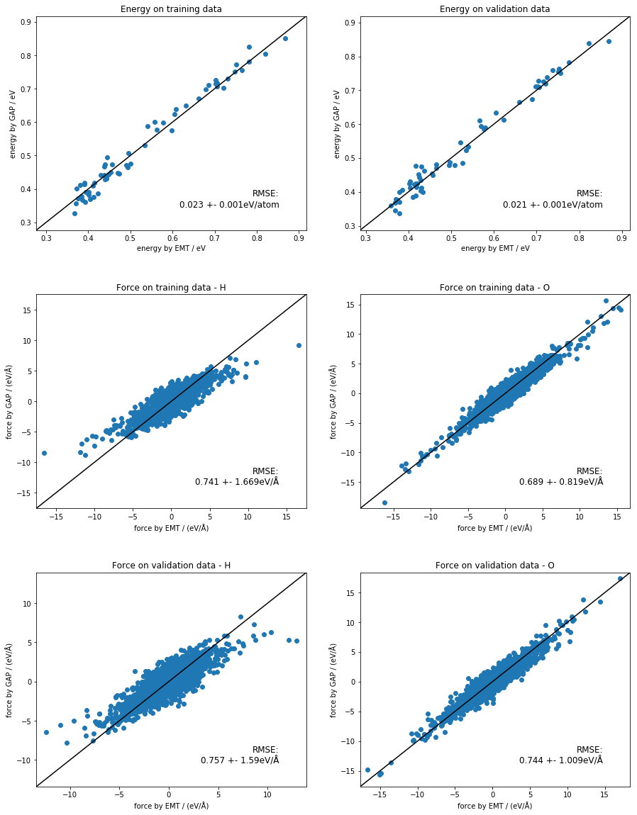
look at the outputs - clear improvement
[26]:
fig, ax_list = plt.subplots(nrows=3, ncols=2, gridspec_kw={'hspace': 0.3})
fig.set_size_inches(15, 20)
ax_list = ax_list.flat[:]

energy_plot('train.xyz', 'quip_3b_train.xyz', ax_list[0], 'Energy on training data')
energy_plot('validate.xyz', 'quip_3b_validate.xyz', ax_list[1], 'Energy on validation data')
force_plot('train.xyz', 'quip_3b_train.xyz', ax_list[2], 'H', 'Force on training data - H')
force_plot('train.xyz', 'quip_3b_train.xyz', ax_list[3], 'O', 'Force on training data - O')
force_plot('validate.xyz', 'quip_3b_validate.xyz', ax_list[4], 'H', 'Force on validation data - H')
force_plot('validate.xyz', 'quip_3b_validate.xyz', ax_list[5], 'O',  'Force on validation data - O')

# if you wanted to have the same limits on the firce plots
#for ax in ax_list[2:]:
#    flim = (-20, 20)
#    ax.set_xlim(flim)
#    ax.set_ylim(flim)
[ ]: