One-dimensional Poisson-Nernst-Planck systems
The matscipy.electrochemistry.PoissonNernstPlanckSystem solver provides an interface for solving classical, one-dimensional electrochemical systems with an arbitrary number of \(N\) ionic species by means of a controlled-volumes method.
The inert electrode
An archetypical system is the inert electrode at the open half-space governed by the Poisson equation and \(N\) Nernst-Planck equations with Dirichlet and zero flux’ boundary conditions as shown in Figure 1 below.

Figure 1: Inert electrode at the open half-space
Here, \(D_i\) is the diffusivity of the ith species, \(c_i\) its local concentration, \(c_i^\infty\) its bulk concentration, \(u_i\) its electric mobility, and \(z_i\) its charge number. \(\phi\) is the local electrostatic potential, and \(\phi_0\) the electrode’s potential compared to the bulk solution. \(\epsilon_0\) is the vacuum permittivity, \(\epsilon_r\) is the relative permittivity of the solvent, and \(F\) is the Faraday constant.
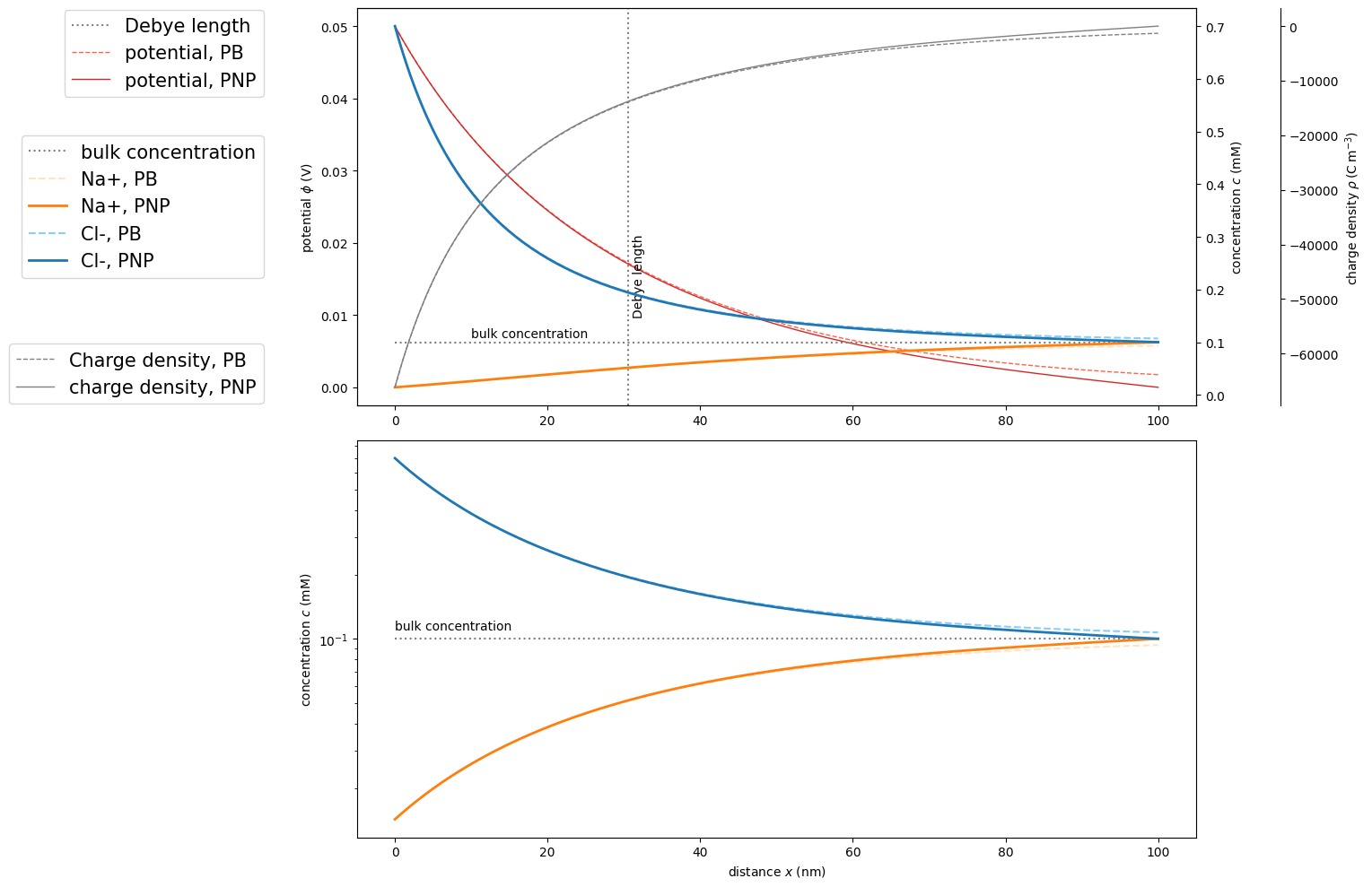
In the following, we use matscipy.electrochemistry.PoissonNernstPlanckSystem to solve this system for \(0.1\,\mathrm{mM}~\text{NaCl}\) at \(0.05\,\mathrm{V}\) bias. Parameters are provided in SI units. We will compare the results against the analytical solution, which exists for this special case of a binary electrolyte.
Preparations
First, we import a few basic tools.
import numpy as np
import scipy.constants as sc
import matplotlib.pyplot as plt
Then, we import the Poisson-Nernst-Planck solver.
from matscipy.electrochemistry import PoissonNernstPlanckSystem
Solving with Dirichlet and zero flux boundary conditions
c = [0.1, 0.1] # bulk concentrations of ion species Na and Cl in mM
z = [1, -1] # number charges of ion species
L = 1e-07 # interval length in m
delta_u = 0.05
The log output of the system’s initialization will show all provided and derived parameters such as the discretization grid as well as their dimensionless values.
pnp = PoissonNernstPlanckSystem(c=c, z=z, L=L, delta_u=delta_u)
The method use_standard_interface_bc will apply boundary conditions as shown in Figure 1, with Dirichlet boundary conditions on the potential and zero total flux boundary conditions on ion diffusion and electromigration.
pnp.use_standard_interface_bc()
ui, nij, _ = pnp.solve()
ui holds the electrostatic potential at the discretization points and nij the species concentrations at the discretization points.
Validation: Analytical half-space solution vs. numerical finite-interval PNP system
matscipy.electrochemistry provides a function for quickly retrieving the Debye length \(\lambda_D\) of an electrolyte.
from matscipy.electrochemistry import debye
deb = debye(c, z)
The analytical solution for the open half-space at an inert electrode is just the Possion-Boltzmann distribution [3]. matscipy.electrochemistry.poisson_boltzmann_distribution provides a few short-hand functions for retrieving electrostatic potential, charge density and concentrations that arise from this analytical solution.
from matscipy.electrochemistry.poisson_boltzmann_distribution import potential, concentration, charge_density

x = np.linspace(0, L, 100)
phi = potential(x, c, z, delta_u)
C =   concentration(x, c, z, delta_u)
rho = charge_density(x, c, z, delta_u)
We define a little helper for a prettifying our plot.
def make_patch_spines_invisible(ax):
    ax.set_frame_on(True)
    ax.patch.set_visible(False)
    for sp in ax.spines.values():
        sp.set_visible(False)
Next, we hold analytical Poisson-Boltzmann (PB) results on the infinite half space and numerical Poisson-Nernst-Planck (PNP) results on the limited interval next to each other and are convinced of the solution’s validity.
fig, (ax1,ax4) = plt.subplots(nrows=2,ncols=1,figsize=[16,10])
ax1.axvline(x=deb/sc.nano, label='Debye length', color='grey', linestyle=':')
ax1.text(deb/sc.nano*1.02, 0.01, "Debye length", rotation=90)

ax1.plot(x/sc.nano, phi, marker='', color='tomato', label='potential, PB', linewidth=1, linestyle='--')
ax1.plot(pnp.grid/sc.nano, pnp.potential, marker='', color='tab:red', label='potential, PNP', linewidth=1, linestyle='-')

ax2 = ax1.twinx()
ax2.plot(x/sc.nano, np.ones(x.shape)*c[0], label='bulk concentration', color='grey', linestyle=':')
ax2.text(10, c[0]*1.1, "bulk concentration")

ax2.plot(x/sc.nano, C[0], marker='', color='bisque', label='Na+, PB',linestyle='--')
ax2.plot(pnp.grid/sc.nano, pnp.concentration[0], marker='', color='tab:orange', label='Na+, PNP', linewidth=2, linestyle='-')

ax2.plot(x/sc.nano, C[1], marker='', color='lightskyblue', label='Cl-, PB',linestyle='--')
ax2.plot(pnp.grid/sc.nano, pnp.concentration[1], marker='', color='tab:blue', label='Cl-, PNP', linewidth=2, linestyle='-')

ax3 = ax1.twinx()
# Offset the right spine of ax3.  The ticks and label have already been
# placed on the right by twinx above.
ax3.spines["right"].set_position(("axes", 1.1))

# Having been created by twinx, ax3 has its frame off, so the line of its
# detached spine is invisible. First, activate the frame but make the patch
# and spines invisible.
make_patch_spines_invisible(ax3)

# Second, show the right spine.
ax3.spines["right"].set_visible(True)

ax3.plot(x/sc.nano, rho, label='Charge density, PB', color='grey', linewidth=1, linestyle='--')
ax3.plot(pnp.grid/sc.nano, pnp.charge_density, label='charge density, PNP', color='grey', linewidth=1, linestyle='-')

ax4.semilogy(x/sc.nano, np.ones(x.shape)*c[0], label='bulk concentration', color='grey', linestyle=':')
ax4.text(0, c[0]*1.1, "bulk concentration")
ax4.semilogy(x/sc.nano, C[0], marker='', color='bisque', label='Na+, PB',linestyle='--')
ax4.semilogy(pnp.grid/sc.nano, pnp.concentration[0], marker='', color='tab:orange', label='Na+, PNP', linewidth=2, linestyle='-')

ax4.semilogy(x/sc.nano, C[1], marker='', color='lightskyblue', label='Cl-, PB',linestyle='--')
ax4.semilogy(pnp.grid/sc.nano, pnp.concentration[1], marker='', color='tab:blue', label='Cl-, PNP', linewidth=2, linestyle='-')

ax1.set_ylabel('potential $\phi$ (V)')
ax2.set_ylabel('concentration $c$ (mM)')
ax3.set_ylabel(r'charge density $\rho \> (\mathrm{C}\> \mathrm{m}^{-3})$')
ax4.set_ylabel('concentration $c$ (mM)')
ax4.set_xlabel('distance $x$ (nm)')

ax1.legend(loc='upper right',  bbox_to_anchor=(-0.1,1.02), fontsize=15)
ax2.legend(loc='center right', bbox_to_anchor=(-0.1,0.5),  fontsize=15)
ax3.legend(loc='lower right',  bbox_to_anchor=(-0.1,-0.02), fontsize=15)

fig.tight_layout()
plt.show()
<>:42: SyntaxWarning: invalid escape sequence '\p'
<>:42: SyntaxWarning: invalid escape sequence '\p'
/tmp/ipykernel_3952/1530268794.py:42: SyntaxWarning: invalid escape sequence '\p'
  ax1.set_ylabel('potential $\phi$ (V)')
The electrochemical cell
Another archetypical system is the one-dimensional electrochemical cell governed by flux and Robin boundary conditions as shown below in Figure 2.

Figure 2: One-dimensional electrochemical cell after Bazant [1]
Here, \(i_\text{cell}\) is the total density of Faradaic current through the cell that arises due to \(M\) half-reactions, with \(i_j\) the partial current due to reaction \(j\). \(\nu_{ij}\) is the stochiometric coefficient of species \(i\), and \(n_j\) the number of electrons participating in half-reaction \(j\). \(\lambda_S\) is the width of a compact Stern layer. The assumption of a compact Stern layer [2] reduces the system’s strong nonlinearity close to the electrode and may facilitate convergence.
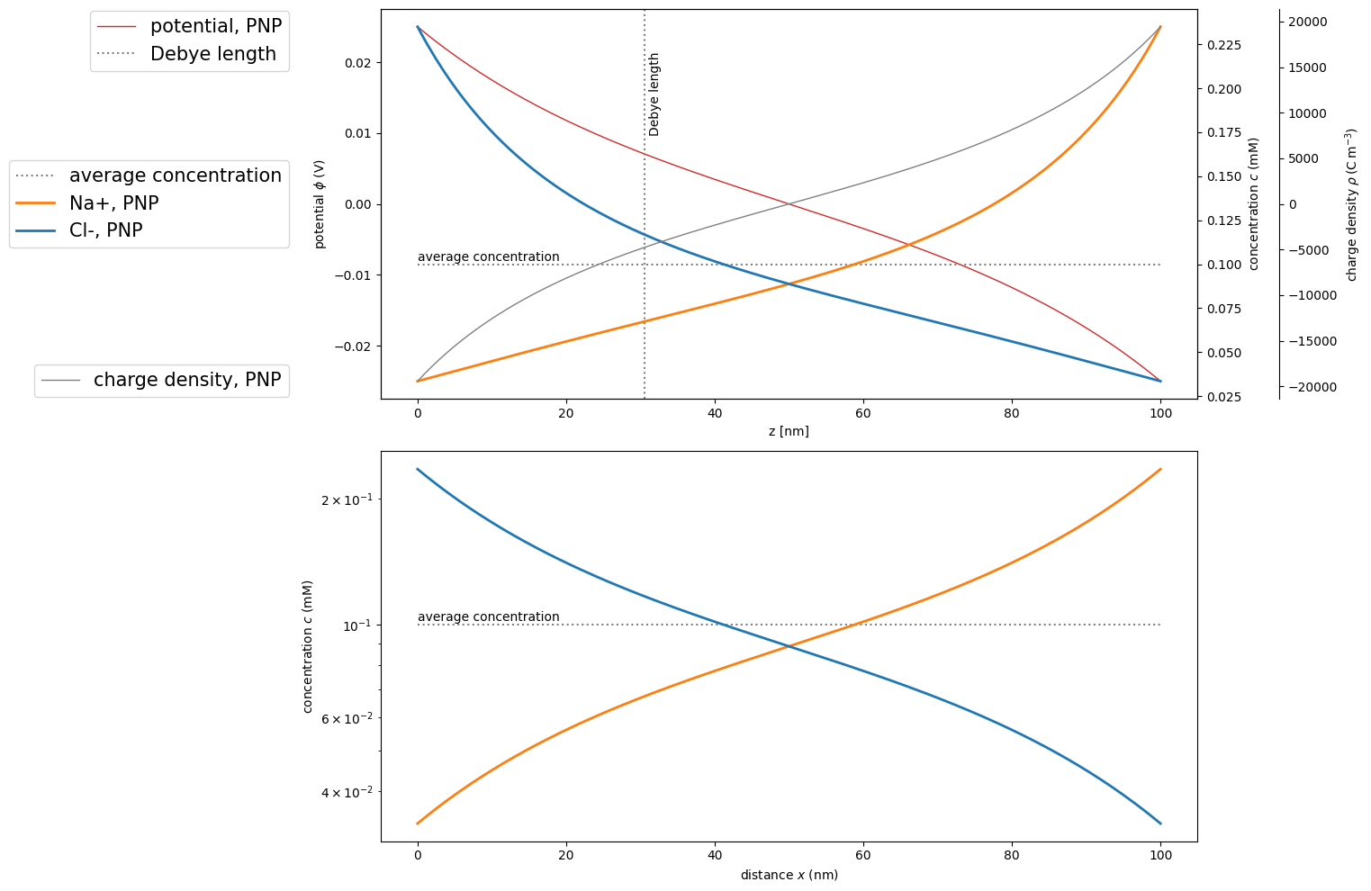
Solving with Dirichlet and zero flux boundary conditions
Again, we solve this system for inert electrodes, i.e. in the absence of any current flux with the same parameters as above.
c = [0.1, 0.1] # bulk concentrations of ion species Na and Cl in mM
z = [1, -1] # number charges of ion species
L = 1e-07 # interval length in m
delta_u = 0.05 # electrostatic potential bias

pnp = PoissonNernstPlanckSystem(c=c, z=z, L=L, delta_u=delta_u)
The only difference is the application of another set of predefined boundary conditions.
pnp.use_standard_cell_bc()
These boundary conditions assume no Stern layer, i.e. \(\lambda_S = 0\)
pnp.output = True
xij = pnp.solve()
Visualization
We show the results in the familiar manner.
x = np.linspace(0, L, 100)

deb = debye(c, z)

fig, (ax1,ax4) = plt.subplots(nrows=2,ncols=1,figsize=[16,10])
ax1.set_xlabel('z [nm]')
ax1.plot(pnp.grid/sc.nano, pnp.potential, marker='', color='tab:red', label='potential, PNP', linewidth=1, linestyle='-')

ax2 = ax1.twinx()
ax2.plot(x/sc.nano, np.ones(x.shape)*c[0], label='average concentration', color='grey', linestyle=':')
ax2.text(0, c[0]*1.02, "average concentration")

ax2.plot(pnp.grid/sc.nano, pnp.concentration[0], marker='', color='tab:orange', label='Na+, PNP', linewidth=2, linestyle='-')

ax2.plot(pnp.grid/sc.nano, pnp.concentration[1], marker='', color='tab:blue', label='Cl-, PNP', linewidth=2, linestyle='-')
ax1.axvline(x=deb/sc.nano, label='Debye length', color='grey', linestyle=':')
ax1.text(deb/sc.nano*1.02, 0.01, "Debye length", rotation=90)

ax3 = ax1.twinx()
ax3.spines["right"].set_position(("axes", 1.1))
make_patch_spines_invisible(ax3)

ax3.spines["right"].set_visible(True)
ax3.plot(pnp.grid/sc.nano, pnp.charge_density, label='charge density, PNP', color='grey', linewidth=1, linestyle='-')

ax4.semilogy(x/sc.nano, np.ones(x.shape)*c[0], label='average concentration', color='grey', linestyle=':')
ax4.text(0, c[0]*1.02, "average concentration")
ax4.semilogy(pnp.grid/sc.nano, pnp.concentration[0], marker='', color='tab:orange', label='Na+, PNP', linewidth=2, linestyle='-')
ax4.semilogy(pnp.grid/sc.nano, pnp.concentration[1], marker='', color='tab:blue', label='Cl-, PNP', linewidth=2, linestyle='-')

ax1.set_ylabel('potential $\phi$ (V)')
ax2.set_ylabel('concentration $c$ (mM)')
ax3.set_ylabel(r'charge density $\rho \> (\mathrm{C}\> \mathrm{m}^{-3})$')
ax4.set_ylabel('concentration $c$ (mM)')
ax4.set_xlabel('distance $x$ (nm)')

ax1.legend(loc='upper right',  bbox_to_anchor=(-0.1,1.02), fontsize=15)
ax2.legend(loc='center right', bbox_to_anchor=(-0.1,0.5),  fontsize=15)
ax3.legend(loc='lower right',  bbox_to_anchor=(-0.1,-0.02), fontsize=15)

fig.tight_layout()
plt.show()
<>:31: SyntaxWarning: invalid escape sequence '\p'
<>:31: SyntaxWarning: invalid escape sequence '\p'
/tmp/ipykernel_3952/562622314.py:31: SyntaxWarning: invalid escape sequence '\p'
  ax1.set_ylabel('potential $\phi$ (V)')
From continuous double layer theory to discrete coordinate sets
Poisson-Nernst-Planck-System with Stern layer boundary conditions
In this example We want to fill a gap of 5 nm between gold electrodes with 0.2 wt % NaCl aqueous solution, apply a small potential difference and generate an initial configuration for LAMMPS within a cubic box.
box_Ang = np.array([50.,50.,50.]) # Angstrom
box_m = box_Ang*sc.angstrom # meters

vol_AngCube = box_Ang.prod() # Angstrom^3
vol_mCube = vol_AngCube*sc.angstrom**3
With a concentration of 0.2 wt %, we are close to NaCl’s solubility limit in water. We estimate molar concentrations and atom numbers in our box.
weight_concentration_NaCl = 0.2 # wt %
# calculate saline mass density g/cm³
saline_mass_density_kg_per_L  = 1 + weight_concentration_NaCl * 0.15 / 0.20 # g / cm^3, kg / L
# see e.g. https://www.engineeringtoolbox.com/density-aqueous-solution-inorganic-sodium-salt-concentration-d_1957.html

saline_mass_density_g_per_L = saline_mass_density_kg_per_L*sc.kilo

molar_mass_H2O = 18.015 # g / mol
molar_mass_NaCl  = 58.44 # g / mol

cNaCl_M = weight_concentration_NaCl*saline_mass_density_g_per_L/molar_mass_NaCl # mol L^-1

cNaCl_mM = np.round(cNaCl_M/sc.milli) # mM

n_NaCl = np.round(cNaCl_mM*vol_mCube*sc.value('Avogadro constant'))
Nearly \(4\,\mathrm{M}\) of saline solution correspond to about 300 ions of each species in our cubic \(5^3\,\mathrm{nm}^3\) box.
We initialize the system assuming a Stern layer of 5 Å width, close to the order of magnitude of ion size.
Solving with Robin and zero flux boundary conditions
c = [cNaCl_mM,cNaCl_mM]
z = [1,-1]
L = box_m[2]
lambda_S = 5.0e-10 # Stern layer width in m
delta_u  = 0.5
Other than above, we modify a few solver parameters as well.
pnp = PoissonNernstPlanckSystem(c,z,L, lambda_S=lambda_S, delta_u=delta_u, N=200, maxit=20, e=1e-6)
The following applies zero flux and, particularly, Robin boundary conditions as shown in Figure 2.
pnp.use_stern_layer_cell_bc()

pnp.output = True
xij = pnp.solve()
Visualization
x = np.linspace(0, L, 100)

deb = debye(c, z)

fig, (ax1,ax4) = plt.subplots(nrows=2,ncols=1,figsize=[16,10])
ax1.plot(pnp.grid/sc.nano, pnp.potential, marker='', color='tab:red', label='potential, PNP', linewidth=1, linestyle='-')

ax2 = ax1.twinx()
ax2.plot(x/sc.nano, np.ones(x.shape)*c[0], label='average concentration', color='grey', linestyle=':')
ax2.text(1, c[0]*1.5, "average concentration")

ax2.plot(pnp.grid/sc.nano, pnp.concentration[0], marker='', color='tab:orange', label='Na+, PNP', linewidth=2, linestyle='-')

ax2.plot(pnp.grid/sc.nano, pnp.concentration[1], marker='', color='tab:blue', label='Cl-, PNP', linewidth=2, linestyle='-')
ax1.axvline(x=deb/sc.nano, label='Debye length', color='grey', linestyle=':')
ax1.text(deb/sc.nano*1.2, 0.01, "Debye length", rotation=90)

ax3 = ax1.twinx()
ax3.spines["right"].set_position(("axes", 1.1))
make_patch_spines_invisible(ax3)

ax3.spines["right"].set_visible(True)
ax3.plot(pnp.grid/sc.nano, pnp.charge_density, label='charge density, PNP', color='grey', linewidth=1, linestyle='-')

ax4.semilogy(x/sc.nano, np.ones(x.shape)*c[0], label='average concentration', color='grey', linestyle=':')
ax4.text(1, c[0]*1.5, "average concentration")
ax4.semilogy(pnp.grid/sc.nano, pnp.concentration[0], marker='', color='tab:orange', label='Na+, PNP', linewidth=2, linestyle='-')
ax4.semilogy(pnp.grid/sc.nano, pnp.concentration[1], marker='', color='tab:blue', label='Cl-, PNP', linewidth=2, linestyle='-')

ax1.set_ylabel('potential $\phi$ (V)')
ax2.set_ylabel('concentration $c$ (mM)')
ax3.set_ylabel(r'charge density $\rho \> (\mathrm{C}\> \mathrm{m}^{-3})$')
ax4.set_ylabel('concentration $c$ (mM)')
ax4.set_xlabel('distance $x$ (nm)')

ax1.legend(loc='upper right',  bbox_to_anchor=(-0.1,1.02), fontsize=15)
ax2.legend(loc='center right', bbox_to_anchor=(-0.1,0.5),  fontsize=15)
ax3.legend(loc='lower right',  bbox_to_anchor=(-0.1,-0.02), fontsize=15)

fig.tight_layout()
plt.show()
<>:30: SyntaxWarning: invalid escape sequence '\p'
<>:30: SyntaxWarning: invalid escape sequence '\p'
/tmp/ipykernel_3952/1594926341.py:30: SyntaxWarning: invalid escape sequence '\p'
  ax1.set_ylabel('potential $\phi$ (V)')
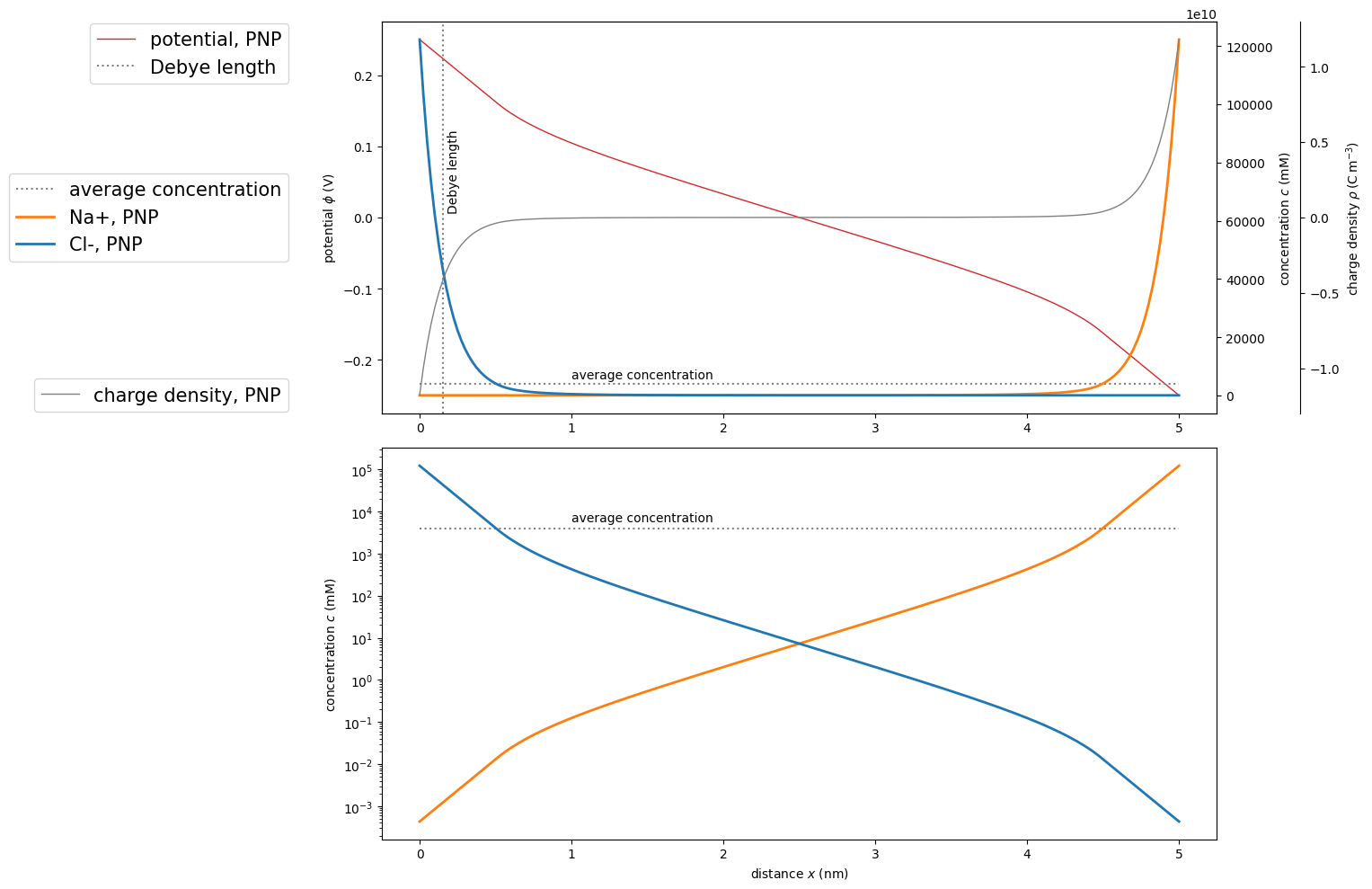
Notice the nearly linear behavior of potential close to the electrodes arising from the Robin boundary conditions.
Sampling from continuous distributions
We want to generate three-dimensional atomistic configurations from the one-dimensional concentration distributions retrieved above. matscipy.electrochemistry provides the sampling interface continuous2discrete for this purpose.
from matscipy.electrochemistry import continuous2discrete
continuous2discrete expects a callable distribution function. Hence, we convert the physical concentration distributions into callable density functions.
from scipy import interpolate
distributions = [interpolate.interp1d(pnp.grid,pnp.concentration[i,:]) for i in range(pnp.concentration.shape[0])]
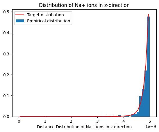
Normalization is not necessary here. Now we can sample the distribution of our \(Na^+\) ions in z-direction.
na_coordinate_sample = continuous2discrete(distribution=distributions[0], box=box_m, count=n_NaCl)
matscipy.electrochemistry provides the utility function get_histogram to count coordinate sets within bins along all three spatial dimensions.
from matscipy.electrochemistry import get_histogram
histx, histy, histz = get_histogram(na_coordinate_sample, box=box_m, n_bins=51)
For visualization purposes, we define two little helper functions.
# helper functions
def get_centers(bins):
    """Return the center of the provided bins.

    Example:
    >>> get_centers(bins=np.array([0.0, 1.0, 2.0]))
    array([ 0.5,  1.5])
    """
    bins = bins.astype(float)
    return (bins[:-1] + bins[1:]) / 2

def plot_dist(histogram, name, reference_distribution=None):
    """Plot histogram with an optional reference distribution."""
    hist, bins = histogram
    width = 1 * (bins[1] - bins[0])
    centers = get_centers(bins)

    fi, ax = plt.subplots()
    ax.bar( centers, hist, align='center', width=width, label='Empirical distribution',
            edgecolor="none")

    if reference_distribution is not None:
        ref = reference_distribution(centers)
        ref /= sum(ref)
        ax.plot(centers, ref, color='red', label='Target distribution')

    ax.set_title(name)
    ax.legend()
    ax.set_xlabel('Distance ' + name)
Eventually, we show the distribution of samples sodium ions along the non-uniform z-direction.
plot_dist(histz, 'Distribution of Na+ ions in z-direction', reference_distribution=distributions[0])
Similarly, we sample chlorine ions…
cl_coordinate_sample = continuous2discrete(distributions[1], box=box_m, count=n_NaCl)
… and show their distribution …
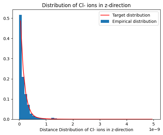
histx, histy, histz = get_histogram(cl_coordinate_sample, box=box_m, n_bins=51)
plot_dist(histx, 'Distribution of Cl- ions in x-direction', reference_distribution=lambda x: np.ones(x.shape)*1/box_m[0])
plot_dist(histy, 'Distribution of Cl- ions in y-direction', reference_distribution=lambda x: np.ones(x.shape)*1/box_m[1])
plot_dist(histz, 'Distribution of Cl- ions in z-direction', reference_distribution=distributions[1])
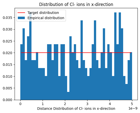
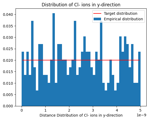
Notice the uniform distribution along x- and y-direction.
Coordinates export
Eventually, we use ASE to export our sample to some standard format, i.e. .xyz or LAMMPS data file.
import ase
import ase.io
ASE speaks Ångström per default, thus we convert our SI units:
sample_size = int(n_NaCl)

na_atoms = ase.Atoms(
    symbols='Na'*sample_size,
    charges=[1]*sample_size,
    positions=na_coordinate_sample/sc.angstrom,
    cell=box_Ang,
    pbc=[1,1,0])

cl_atoms = ase.Atoms(
    symbols='Cl'*sample_size,
    charges=[-1]*sample_size,
    positions=cl_coordinate_sample/sc.angstrom,
    cell=box_Ang,
    pbc=[1,1,0])

system = na_atoms + cl_atoms

ase.io.write('NaCl_c_4_M_u_0.5_V_box_5x5x5nm_lambda_S_5_Ang.xyz', system, format='xyz')

# LAMMPS data format, units 'real', atom style 'full'
# before ASE 3.19.0b1, ASE had issues with exporting atom style 'full' in LAMMPS data file format, so do not expect this line to work for older ASE versions
ase.io.write('NaCl_c_4_M_u_0.5_V_box_5x5x5nm_lambda_S_5_Ang.lammps', system,
             format='lammps-data', units="real", atom_style='full')
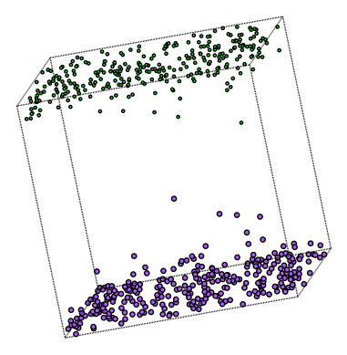
Looking at the configuration, most ions are found within a Debye length next to the electrodes.
import matplotlib.pyplot as plt
from ase.visualize.plot import plot_atoms
fig, ax = plt.subplots()
plot_atoms(system, ax, radii=0.3, rotation=('80x,10y,10z'))
ax.set_axis_off()
References
[1] M. Z. Bazant, K. T. Chu, and B. J. Bayly, “Current-Voltage Relations for Electrochemical Thin Films,” SIAM Journal on Applied Mathematics, Jul. 2006, doi: 10.1137/040609938.
[2] O. Stern, “Zur Theorie Der Elektrolytischen Doppelschicht,” Zeitschrift für Elektrochemie und angewandte physikalische Chemie, vol. 30, no. 21–22, pp. 508–516, 1924, doi: 10.1002/bbpc.192400182.
[3] J. N. Israelachvili, Intermolecular and surface forces. Academic Press, London, 1991.