Steric correction

Continuum models do not account for the finite size of atoms. Sampling discrete particle coordinates from continuous concentration distributions may thus result in arbitrarily close atom positions. To avoid overlap and yield usable atomistic configurations from densely packed samples, matscipy.electrochemistry offers the steric_correction sub-module. Its function apply_steric_correction applies a steric correction to the provided configuration, assuring the desired steric radii for all species if possible. To achieve this, the module re-implements a pseudo-potential minimization algorithm [1] used by PACKMOL in Python

Below, we generate continuous concentration distributions from classical electrochemical double layer theory, sample coordinates from these distributions, and apply a steric correction to the ion coordinates.

Theory and mechanisms involved in step 1 and 2 have been discussed in detail in previous documentation sections.

Step 1: generating continuous concentration distributions

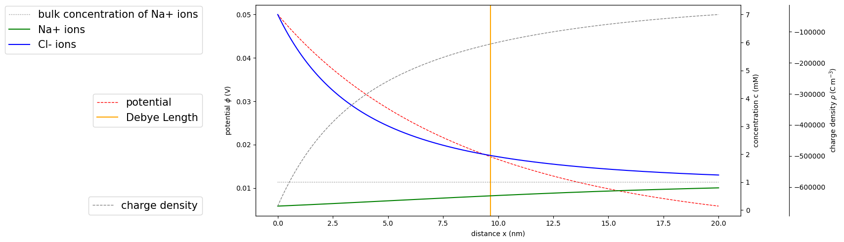
Adjacent to an inert electrode at an open half-space, concentration distributions of a binary electrolyte are retrieved from the analytical solution of the Poisson-Boltzmann equation. matscipy.electrochemistry.poisson_boltzmann_distribution provides a simple interface to this analytical solution. Let’s consider 1 mM saline solution.

from matscipy.electrochemistry.poisson_boltzmann_distribution import (
    potential, concentration, charge_density)

/usr/lib/python3/dist-packages/scipy/__init__.py:146: UserWarning: A NumPy version >=1.17.3 and <1.25.0 is required for this version of SciPy (detected version 1.26.4
  warnings.warn(f"A NumPy version >={np_minversion} and <{np_maxversion}"

Although we look at a continuous 1d system now, we want to sample coordinates in a 3d box from it later. Hence, we specify the 3d box size here already and retrieve potential, concentration and charge distributions arising from solving the Poisson-Boltzmann equation analytically.

import numpy as np 

# measures of box
xsize = ysize = 5e-9 # nm, SI units
zsize = 20e-9        # nm, SI units

x = np.linspace(0, zsize, 2000)
c = [1, 1]   # bulk concentrations of Na and Cl, mM, SI units
z = [1, -1]  # number charges of species
u = 0.05     # electrostatic potential across the interface, V

phi = potential(x, c, z, u)
C   = concentration(x, c, z, u)
rho = charge_density(x, c, z, u)

Next, we visualize these distributions.

import matplotlib.pyplot as plt
import scipy.constants as sc    # fundamental constants

from matscipy.electrochemistry import debye

def make_patch_spines_invisible(ax):
    ax.set_frame_on(True)
    ax.patch.set_visible(False)
    for sp in ax.spines.values():
        sp.set_visible(False)
        

deb = debye(c, z) 

fig, ax1 = plt.subplots(figsize=[18,5])
ax1.set_xlabel('distance x (nm)')
ax1.plot(x/sc.nano, phi, marker='', color='red', label='potential', linewidth=1, linestyle='--')
ax1.set_ylabel('potential $\phi$ (V)')
ax1.axvline(x=deb/sc.nano, label='Debye Length', color='orange')

ax2 = ax1.twinx()
ax2.plot(x/sc.nano, np.ones(x.shape)*c[0], label='bulk concentration of Na+ ions', color='grey', linewidth=1, linestyle=':')
ax2.plot(x/sc.nano, C[0], marker='', color='green', label='Na+ ions')
ax2.plot(x/sc.nano, C[1], marker='', color='blue', label='Cl- ions')
ax2.set_ylabel('concentration c (mM)')

ax3 = ax1.twinx()
# Offset the right spine of par2.  The ticks and label have already been
# placed on the right by twinx above.
ax3.spines["right"].set_position(("axes", 1.1))
# Having been created by twinx, par2 has its frame off, so the line of its
# detached spine is invisible.  First, activate the frame but make the patch
# and spines invisible.
make_patch_spines_invisible(ax3)
# Second, show the right spine.
ax3.spines["right"].set_visible(True)

ax3.plot(x/sc.nano, rho, label='charge density', color='grey', linewidth=1, linestyle='--')
ax3.set_ylabel(r'charge density $\rho \> (\mathrm{C}\> \mathrm{m}^{-3})$')

ax2.legend(loc='upper right', bbox_to_anchor=(-0.1, 1.02),fontsize=15)
ax1.legend(loc='center right', bbox_to_anchor=(-0.1,0.5), fontsize=15)
ax3.legend(loc='lower right', bbox_to_anchor=(-0.1, -0.02), fontsize=15)
fig.tight_layout()
plt.show()

Step 2: sampling from distributions

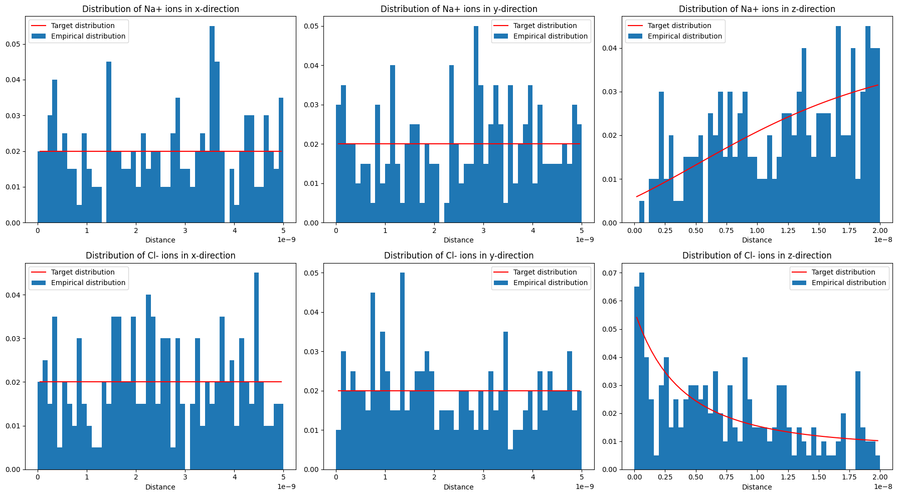
We sample and visualize discrete coordinate sets from our continuous distributions as before.

from scipy import interpolate
from matscipy.electrochemistry import continuous2discrete
from matscipy.electrochemistry import get_histogram

# helper functions
def get_centers(bins):
    """Return the center of the provided bins.

    Example:
    >>> get_centers(bins=np.array([0.0, 1.0, 2.0]))
    array([ 0.5,  1.5])
    """
    bins = bins.astype(float)
    return (bins[:-1] + bins[1:]) / 2

def plot_dist(histogram, name, reference_distribution=None, ax=None):
    """Plot histogram with an optional reference distribution."""
    hist, bins = histogram
    width = 1 * (bins[1] - bins[0])
    centers = get_centers(bins)

    if ax is None:
        _, ax = plt.subplots()
        
    ax.bar( centers, hist, align='center', width=width, label='Empirical distribution',
            edgecolor="none")

    if reference_distribution is not None:
        ref = reference_distribution(centers)
        ref /= sum(ref)
        ax.plot(centers, ref, color='red', label='Target distribution')

    ax.set_title(name)
    ax.legend()
    ax.set_xlabel('Distance')

# create distribution functions
distributions = [interpolate.interp1d(x,c) for c in C]

# sample discrete coordinate set
box3 = np.array([xsize, ysize, zsize])
sample_size = 200

samples = [continuous2discrete(distribution=d, box=box3, count=sample_size) for d in distributions]
species = ['Na+','Cl-']
fig, axes = plt.subplots(2,3,figsize=[18,10])
for ion, sample, d, ax_row in zip(species, samples, distributions, axes):
    histx, histy, histz = get_histogram(sample, box=box3, n_bins=51)
    plot_dist(histx, 'Distribution of {:s} ions in x-direction'.format(ion), 
              reference_distribution=lambda x: np.ones(x.shape)*1/box3[0], ax=ax_row[0])
    plot_dist(histy, 'Distribution of {:s} ions in y-direction'.format(ion), 
              reference_distribution=lambda x: np.ones(x.shape)*1/box3[1], ax=ax_row[1])
    plot_dist(histz, 'Distribution of {:s} ions in z-direction'.format(ion), 
              reference_distribution=d, ax=ax_row[2])

fig.tight_layout()

Step 3: enforcing steric radii

matscipy.electrochemistry.steric_correction exposes a few functions for finding the closest pair within a coordinate set. We use scipy_distance_based_closest_pair to inspect our coordinates in their initial state:

Inspect the initial coordinate sample

from matscipy.electrochemistry.steric_correction import scipy_distance_based_closest_pair

# need all coordinates in one N x 3 array
xstacked = np.vstack(samples)

box6 = np.array([[0.,0.,0], box3]) # needs lower corner

mindsq, (p1,p2) = scipy_distance_based_closest_pair(xstacked)
pmin = np.min(xstacked, axis=0)
pmax = np.max(xstacked, axis=0)
mind = np.sqrt(mindsq)
print("Minimum pair-wise distance in sample: {}".format(mind))
print("First sample point in pair:    ({:8.4e},{:8.4e},{:8.4e})".format(*p1))
print("Second sample point in pair    ({:8.4e},{:8.4e},{:8.4e})".format(*p2))
print("Box lower boundary:            ({:8.4e},{:8.4e},{:8.4e})".format(*box6[0]))
print("Minimum coordinates in sample: ({:8.4e},{:8.4e},{:8.4e})".format(*pmin))
print("Maximum coordinates in sample: ({:8.4e},{:8.4e},{:8.4e})".format(*pmax))
print("Box upper boundary:            ({:8.4e},{:8.4e},{:8.4e})".format(*box6[1]))

Minimum pair-wise distance in sample: 1.352188695855715e-10
First sample point in pair:    (4.4566e-09,3.7113e-09,1.3501e-08)
Second sample point in pair    (4.3269e-09,3.6958e-09,1.3537e-08)
Box lower boundary:            (0.0000e+00,0.0000e+00,0.0000e+00)
Minimum coordinates in sample: (2.3292e-12,6.1885e-13,2.2696e-11)
Maximum coordinates in sample: (4.9992e-09,4.9942e-09,1.9953e-08)
Box upper boundary:            (5.0000e-09,5.0000e-09,2.0000e-08)

The distance between the closest pair of ions will be at the order of an Ångström.

Apply the steric correction

Next, we use apply_steric_correction to ensure a radius of 2 Å on all our ions. If no other method specified, then apply_steric_correction uses scipy’s L-BFGS-B minimizer.

from matscipy.electrochemistry.steric_correction import apply_steric_correction

r = 2e-10 # 2 Angstrom steric radius

x1, res = apply_steric_correction(xstacked, box=box6, r=r, options={'disp': False})

/tmp/ipykernel_8908/3409156327.py:5: DeprecationWarning: `product` is deprecated as of NumPy 1.25.0, and will be removed in NumPy 2.0. Please use `prod` instead.
  x1, res = apply_steric_correction(xstacked, box=box6, r=r, options={'disp': False})

We inspect the results. The minimal pair distance comes close enough to 4 Å now.

mindsq, (p1,p2) = scipy_distance_based_closest_pair(x1)
mind = np.sqrt(mindsq)
pmin = np.min(x1,axis=0)
pmax = np.max(x1,axis=0)

print("scipy-interfaced L-BFGS-B minimizer finished with")
print("    status = {}, success = {}, #it = {}".format(
    res.status, res.success, res.nit))
print("    message = '{}'".format(res.message))
print("")
print("Minimum pair-wise distance in final configuration: {:8.4e}".format(mind))
print("First sample point in pair:    ({:8.4e},{:8.4e},{:8.4e})".format(*p1))
print("Second sample point in pair    ({:8.4e},{:8.4e},{:8.4e})".format(*p2))
print("Box lower boundary:            ({:8.4e},{:8.4e},{:8.4e})".format(*box6[0]))
print("Minimum coordinates in sample: ({:8.4e},{:8.4e},{:8.4e})".format(*pmin))
print("Maximum coordinates in sample: ({:8.4e},{:8.4e},{:8.4e})".format(*pmax))
print("Box upper boundary:            ({:8.4e},{:8.4e},{:8.4e})".format(*box6[1]))

scipy-interfaced L-BFGS-B minimizer finished with
    status = 0, success = True, #it = 9
    message = 'CONVERGENCE: NORM_OF_PROJECTED_GRADIENT_<=_PGTOL'

Minimum pair-wise distance in final configuration: 3.9730e-10
First sample point in pair:    (7.2318e-10,3.7182e-10,9.2865e-09)
Second sample point in pair    (9.4771e-10,2.8167e-10,9.6017e-09)
Box lower boundary:            (0.0000e+00,0.0000e+00,0.0000e+00)
Minimum coordinates in sample: (2.0979e-10,2.0107e-10,2.2803e-10)
Maximum coordinates in sample: (4.7982e-09,4.7956e-09,1.9780e-08)
Box upper boundary:            (5.0000e-09,5.0000e-09,2.0000e-08)

Out of 400 positions, that many have been shifted:

# Check difference between initial and final configuration
np.count_nonzero(xstacked - x1) # that many coordinates modified

353

# Check difference between initial and final configuration
np.linalg.norm(xstacked - x1) # euclidean distance between two sets

7.96192377352509e-09

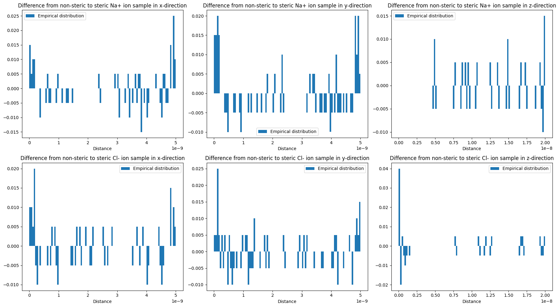
Visualize the applied corrections

# pick last result and split by species
steric_samples = [x1[:sample_size,:], x1[sample_size:,:]]

# Distribution of corrections
fig, axes = plt.subplots(2, 3, figsize=[18, 10])

n_bins = 101
for ion, sample, steric_sample, d, ax_row in zip(species, samples, steric_samples, distributions, axes):

    hists = get_histogram(sample, box=box3, n_bins=n_bins)    
    steric_hists = get_histogram(steric_sample, box=box3, n_bins=n_bins)    
    
    # first entry is counts, second entry is bins
    diff_hists = [(h[0] - hs[0], h[1]) for h,hs in zip(hists, steric_hists)]
    
    for ax, h, ax_col in zip(['x','y','z'], diff_hists, ax_row):
        plot_dist(h, 'Difference from non-steric to steric {:s} ion sample in {:s}-direction'.format(ion, ax), ax=ax_col)

fig.tight_layout()

Export initial and steric configurations

We may use ASE to export both initial and steric coordinate samples to LAMMPS data files.

import ase
import ase.io

symbols = ['Na','Cl']

system = ase.Atoms(
    cell=np.diag(box3/sc.angstrom),
    pbc=[True,True,False]) 

for symbol, sample, charge in zip(symbols, samples, z):
    system += ase.Atoms(
        symbols=symbol*sample_size,
        charges=[charge]*sample_size,
        positions=sample/sc.angstrom)

steric_system = ase.Atoms(
    cell=np.diag(box3/sc.angstrom),
    pbc=[True,True,False]) 

for symbol, sample, charge in zip(symbols, steric_samples, z):
    steric_system += ase.Atoms(
        symbols=symbol*sample_size,
        charges=[charge]*sample_size,
        positions=sample/sc.angstrom)

ase.io.write('NaCl_200_0.05V_5x5x20nm_at_interface_pb_distributed.lammps',
             system,format='lammps-data', units="real", atom_style='full')
ase.io.write('NaCl_200_0.05V_5x5x20nm_at_interface_pb_distributed_steric_correction_2Ang.lammps',
             steric_system, format='lammps-data', units="real", atom_style='full')

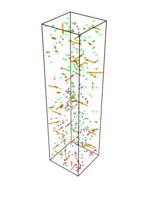
The following visualization of the applied coordinate shifts has been created by showing displacement vectors between non-steric and steric sample with Ovito:

References

[1] L. Martinez, R. Andrade, E. G. Birgin, and J. M. Martínez, “PACKMOL: A package for building initial configurations for molecular dynamics simulations,” J. Comput. Chem., vol. 30, no. 13, pp. 2157–2164, 2009, doi: 10.1002/jcc.21224.