Step 2: Classical MD simulation of fracture in Si

This part of the tutorial requires the initial crack structure crack.xyz produced in Step 1: Setup of the Silicon model system. If you had problems completing the first part, you can download it here instead. Start by creating a new empty script, named run_crack_classical.py.

2.1 Initialisation of the atomic system (20 minutes)

Import the relevant modules

As before, we import the necessary modules, classes and functions:

import numpy as np

from ase.constraints import FixAtoms
from ase.md.verlet import VelocityVerlet
from ase.md.velocitydistribution import MaxwellBoltzmannDistribution
import ase.units as units

from quippy.atoms import Atoms
from quippy.potential import Potential
from quippy.io import AtomsWriter

from quippy.crack import (get_strain,
                          get_energy_release_rate,
                          ConstantStrainRate,
                          find_crack_tip_stress_field)

Note that the molecular dynamics classes and functions come from ASE, while the Atoms object, potentials and crack-specific functionality come from quippy.

Definition of the simulation parameters

Let’s define the simulation parameters. The meaning of each parameter is explained in the comments on the right of each line:

input_file = 'crack.xyz'         # File from which to read crack slab structure
sim_T = 300.0*units.kB           # Simulation temperature
nsteps = 10000                   # Total number of timesteps to run for
timestep = 1.0*units.fs          # Timestep (NB: time base units are not fs!)
cutoff_skin = 2.0*units.Ang      # Amount by which potential cutoff is increased
                                 # for neighbour calculations
tip_move_tol = 10.0              # Distance tip has to move before crack
                                 # is taken to be running
strain_rate = 1e-5*(1/units.fs)  # Strain rate
traj_file = 'traj.nc'            # Trajectory output file (NetCDF format)
print_interval = 10              # Number of time steps between
                                 # writing output frames
param_file = 'params.xml'        # Filename of XML file containing
                                 # potential parameters
mm_init_args = 'IP SW'           # Initialisation arguments for
                                 # classical potential

Setup of the atomic structure

As a first step, we need to initialise the Atoms object by loading the atomic structure created in Step 1: Setup of the Silicon model system from the input_file crack.xyz. Note that the global fortran_indexing setting should be set to False. Otherwise quippy uses atom indices in the range \(1 \ldots N\), which would not be consistent with the python indexing used in ASE (\(0\ldots N-1\)).

It is also necessary to read in the original width and height of the slab and the original crack position, which were saved in crack.xyz at the end of Step 1:

print 'Loading atoms from file %s' % input_file
atoms = ...                                     # Load atoms from file

orig_height = atoms.info['OrigHeight']          # Initialise original height
orig_crack_pos = atoms.info['CrackPos'].copy()  # Initialise original crack position

Note that we make a copy of the CrackPos entry in the info dictionary, since otherwise orig_crack_pos would continue to refer to the current crack position as it is updated during the dynamical simulation.

Setup of the constraints

Now we can set constraints on the atomic structure which will be enforced during dynamics. In order to carry out the fracture MD simulation, we need to fix the positions of the top and bottom atomic rows (we call this constraint fix_atoms).

The fix_atoms constraint, which is exactly the same as the constraint used for relaxing the positions of the crack slab above. In order to do this, we need to find the y coordinate of the top, bottom atomic rows. The x coordinates of the left and right edges of the slab might also be useful later on. This can be easily done as before:

top = ...     # Maximum y coordinate
bottom = ...  # Minimum y coordinate
left = ...    # Minimum x coordinate
right = ...   # Maximum x coordinate

Now it is possible to define the fixed_mask array, which is True for each atom whose position needs to be fixed, and False otherwise, exactly as before, and to initialise the fix_atoms constraint, in the same way we did it in Step 1 (i.e., using the FixAtoms class):

fixed_mask = ...                             # Define the list of fixed atoms
fix_atoms = ...                              # Initialise the constraint
print('Fixed %d atoms\n' % fixed_mask.sum()) # Print the number of fixed atoms

This constraint needs to be attached to our atoms object (see set_constraint()):

atoms. ...  # Attach the constraints to atoms

To increase \(\epsilon_{yy}\) of all atoms at a constant rate (see the strain_rate and timestep parameters), we use the ConstantStrainRate class:

strain_atoms = ConstantStrainRate(orig_height, strain_rate*timestep)

You can look at the documentation for the ConstantStrainRate class to see how this works. The adjust_positions() routine simply increases the strain of all atoms. We will attach this to the dynamics in step 2.2 below.

Setup of the potential

Before starting the MD simulation, the SW classical potential must be initialised and attached to the atoms object. As in Step 1, we use quippy’s Potential class, but now we need to pass the cutoff_skin parameter, which is used to decide when the neighbour list needs to be updated (see the attribute cutoff_skin). Moreover, we request the potential to compute per-atom stresses whenever we compute forces using set_default_quantities(), to save time when locating the crack tip (discussed in more detail below). The set_calculator() method should then be used to set the calculator to the SW potential:

mm_pot = ...   # Initialise the SW potential with cutoff_skin
mm_pot.set_default_quantities(['stresses'])
atoms. ...     # Set the calculator

Milestone 2.1

At this stage your script should look something like this.

2.2 Setup and run the classical MD (20 minutes)

Setting initial velocities and constructing the dynamics object

There are still a few things that need to be done before running the MD fracture simulation. We will follow the standard ASE molecular dynamics methodology. We will set the initial temperature of the system to 2*sim_T: it will then equilibrate to sim_T, by the Virial theorem:

MaxwellBoltzmannDistribution(atoms, 2.0*sim_T)

A MD simulation in the NVE ensemble, using the Velocity Verlet algorithm, can be initialised with the ASE VelocityVerlet class, which requires two arguments: the atoms and the time step (which should come from the timestep parameter:

dynamics = ...   # Initialise the dynamics

Printing status information

Let’s also define a function that prints the relevant information at each time step of the MD simulation. The information can be saved inside the info dictionary, so that it also gets saved to the trajectory file traj_file.

The elapsed simulation time can be obtained with dynamics.get_time() (note that the time unit in ASE is \(\mathrm{\AA}\sqrt{\mathrm{amu}/\mathrm{eV}}\), not fs). You should use the get_kinetic_energy() method to calculate the temperature (Note: you will need the units.kB constant, which gives the value of the Boltzmann constant in eV/K), and the functions get_strain() and get_energy_release_rate() to return the current strain energy release rate, respectively.

def printstatus():
    if dynamics.nsteps == 1:
        print """
State      Time/fs    Temp/K     Strain      G/(J/m^2)  CrackPos/A D(CrackPos)/A
---------------------------------------------------------------------------------"""

    log_format = ('%(label)-4s%(time)12.1f%(temperature)12.6f'+
        '%(strain)12.5f%(G)12.4f%(crack_pos_x)12.2f    (%(d_crack_pos_x)+5.2f)')

    atoms.info['label'] = 'D'                # Label for the status line
    atoms.info['time'] = ...                 # Get simulation time
                                             # and convert to fs
    atoms.info['temperature'] = ...          # Get temperature in K
    atoms.info['strain'] = ...               # Get strain
    atoms.info['G'] = ...                    # Get energy release rate,
                                             # and convert to J/m^2
    crack_pos = ...                          # Find crack tip as in step 1
    atoms.info['crack_pos_x'] = crack_pos[0]
    atoms.info['d_crack_pos_x'] = crack_pos[0] - orig_crack_pos[0]

    print log_format % atoms.info

This logger can be now attached to the dynamics, so that the information is printed at every time step during the simulations:

dynamics.attach(printstatus)

Checking if the crack has advanced

The same can be done to check during the simulation if the crack has advanced, and to stop incrementing the strain if it has:

def check_if_cracked(atoms):
    crack_pos = ...                          # Find crack tip position

    # stop straining if crack has advanced more than tip_move_tol
    if not atoms.info['is_cracked'] and (crack_pos[0] - orig_crack_pos[0]) > tip_move_tol:
        atoms.info['is_cracked'] = True
        del atoms.constraints[atoms.constraints.index(strain_atoms)]

The check_if_cracked function can now be attached to the dynamical system, requesting an interval of 1 step (i.e. every time) and passing the atoms object along to the function as an extra argument:

dynamics.attach(check_if_cracked, 1, atoms)

We also need to attach the :meth:`quippy.crack.ConstrainStrainRate.apply_strain method of strain_atoms to the dynamics:

dynamics.attach(strain_atoms.apply_strain, 1, atoms)

Saving the trajectory

Finally, we need to initialise the trajectory file traj_file and to save frames to the trajectory every traj_interval time steps. This is done by creating a trajectory object with the AtomsWriter() function, and then attaching this trajectory to the dynamics:

trajectory = ...    # Initialise the trajectory
dynamics. ...       # Attach the trajectory with an interval of
                    # traj_interval, passing atoms as an extra argument

We will save the trajectory in netcdf format. This is a binary file format that is similar with the extendedxyz format we used earlier, with the advantage of being more efficient for large files.

Running the dynamics

After all this, a single command will run the MD for nsteps (see the ASE molecular dynamics methodology for more information):

dynamics.run(nsteps)

Milestone 2.2

If you have problems you can look at the complete version of the Step 2 solution — run_crack_classical.py script. Leave your classical MD simulation running and move on to the next section of the tutorial.

The first few lines produced by the run_crack_classical.py script should look something like this:

Loading atoms from file crack.xyz
Fixed 240 atoms


State      Time/fs    Temp/K     Strain      G/(J/m^2)  CrackPos/A D(CrackPos)/A
---------------------------------------------------------------------------------
D            1.0  560.097755     0.08427      5.0012      -30.61    (-0.00)
D            2.0  550.752265     0.08428      5.0024      -30.61    (-0.00)
D            3.0  535.568949     0.08429      5.0036      -30.61    (-0.00)
D            4.0  515.074874     0.08430      5.0047      -30.61    (-0.00)
D            5.0  489.977973     0.08431      5.0059      -30.61    (-0.00)
D            6.0  461.140488     0.08432      5.0071      -30.61    (-0.00)
D            7.0  429.546498     0.08433      5.0083      -30.61    (-0.00)
D            8.0  396.264666     0.08434      5.0095      -30.61    (-0.01)
D            9.0  362.407525     0.08435      5.0107      -30.61    (-0.01)
D           10.0  329.088872     0.08436      5.0119      -30.61    (-0.01)

Here we see the current time, temperature, strain, energy release rate G, the x coordinate of the crack position, and the change in the crack position since the beginning of the simulation. In the early stages of the calculation, the strain and G are both increasing, and the temperature is rapidly falling towards sim_T = 300 as anticipated.

2.3 Visualisation and Analysis (as time permits)

Start another ipython session is a new terminal with plotting support enabled, using the shell command:

ipython --pylab

This will allow you to look at the progress of your classical fracture simulation while it continues to run. All the example code given in this section should be entered directly at the ipython prompt.

The first step is to import everything from quippy using the qlab interactive module, then open your trajectory using the view() function:

from qlab import *
set_fortran_indexing(False)
view("traj.nc")

As we saw earlier, this will open an AtomEye viewer window containing a visual representation of your crack system (as before fortran_indexing=False is used to number the atoms starting from zero). You can use the Insert and Delete keys to move forwards or backwards through the trajectory, or Ctrl+Insert and Ctrl+Delete to jump to the first or last frame – note that the focus must be on the AtomEye viewer window when you use any keyboard shortcuts. The current frame number is shown in the title bar of the window.

The function gcat() (short for “get current atoms”) returns a reference to the Atoms object currently being visualised (i.e. to the current frame from the trajectory file). Similarly, the gcv() function returns a reference to the entire trajectory currently being viewed as an AtomsReaderViewer object.

You can change the frame increment rate by setting the delta attribute of the viewer, e.g. to advance by ten frames at a time:

set_delta(10)

Or, to jump directly to frame 100:

set_frame(100)

You can repeat the view("traj.nc") command as your simulation progresses to reload the file (you can use Ctrl+R in the ipython console to search backwards in the session history to save typing).

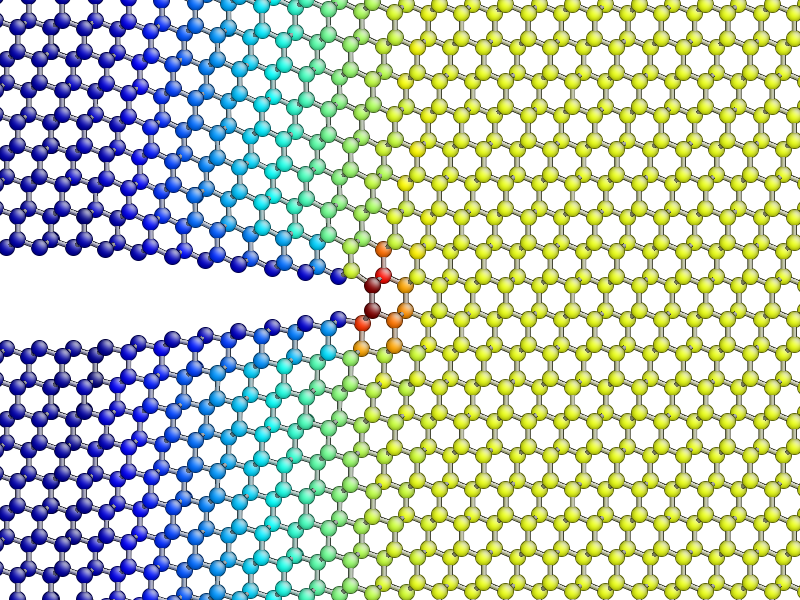
Stress field analysis

To compute and display the instantaneous principal per-atom stress \(\sigma_{yy}\) as computed by the SW potential for a configuration near the beginning of your dynamical simulation:

mm_pot = Potential('IP SW', param_filename='params.xml')
at = gcat()
at.set_calculator(mm_pot)
mm_sigma = at.get_stresses()
sigma_yy = mm_sigma[:,1,1]
aux_property_coloring(sigma_yy)

The mm_sigma array has shape (len(atoms), 3, 3), i.e. it is made up of a \(3 \times 3\) stress tensor \(\sigma_{ij}\) for each atom. The sigma_yy array is the [1, 1] component of each of these arrays, i.e. \(\sigma_{yy}\). To read off the value of the stress on a particular atom, just right click on it. As before, this prints various information in the ipython console. The _show property corresponds to the values currently being used to colour the atoms. You will see that \(\sigma_{yy}\) is very strongly peaked near the crack tip. If you prefer to see the values in GPa, you could do

aux_property_coloring(sigma_yy/units.GPa)

The concept of per-atom stresses is a little arbitrary. The values we are plotting here were obtained from partitioning the total virial stress tensor, which is given by

\[\begin{split}\tau_{ij} = \frac{1}{\Omega} \sum_{k \in \Omega} (-m^{(k)} (u_i^{(k)}- \bar{u}_i) (u_j^{(k)}- \bar{u}_j) %\\ + \frac{1}{2} \sum_{\ell \in \Omega} ( x_i^{(\ell)} - x_i^{(k)}) f_j^{(k\ell)} )\end{split}\]

where \(k\) and \(l\) are atom indices, \(ijk\) are Cartesian indicies, \(\Omega\) is the cell volume, \(m^{(k)}\), \(u^{(k)}\), \(x^{(k)}\) and \(f^{(k)}\) are respectively the mass, velocity, position of atom \(k\) and \(f^{kl}_j\) is the \(j\)th component of the force between atoms \(k\) and \(l\). The first term is a kinetic contribution which vanishes at near zero temperature, and it is common to use the second term to define a per-atom stress tensor.

Note, however, that this requires a definition of the atomic volume. By default the get_stresses() function simply divides the total cell volume by the number of atoms to get the volume per atom. This is not a very good approximation for our cell, which contains a lot of empty vacuum, so the volume per atom comes out much too large, and the stress components much too small, e.g. the peak stress, which you can print in units of GPa with:

print mm_sigma.max()/units.GPa

is around 4 GPa. Values of stress in better agreement with linear elastic theory can be obtained by assuming all atoms occupy the same volume as they would in the equilibrium bulk structure:

mm_pot.set(vol_per_atom=si_bulk.get_volume()/len(si_bulk))
mm_sigma = at.get_stresses()
print mm_sigma.max()/units.GPa

gives a value of around 25 GPa. As this is only a simple rescaling, the unscaled virial stress values are perfectly adequate for locating the crack tip.

Use values from the sigma_yy array to plot the \(\sigma_{yy}\) virial stress along the line \(y=0\) ahead of the crack tip, and verify the stress obeys the expected \(1/\sqrt{r}\) divergence near the crack tip, and tends to a constant value ahead of the crack, due to the thin strip loading. Hint: use a mask to select the relevant atoms, as we did when fixing the edge atoms above. You can use the matplotlib plot() function to produce a plot.

Time-averaged stress field

By now, you should have a few picoseconds of dynamics in your trajectory file. Reload with view("traj.nc") to see what is happening. You can jump to the end with Ctrl+Delete, or by typing last() into the ipython console. Here is what the instantaneous \(\sigma_{yy}\) looks like after 5 ps of dynamics:

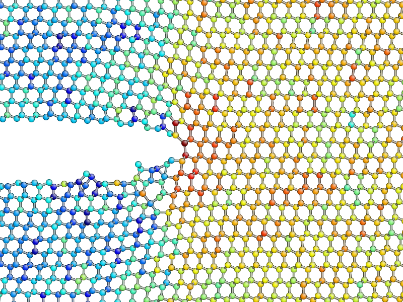
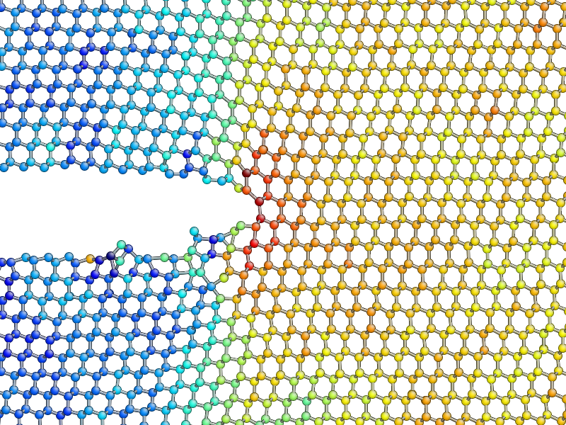
As you can see, the stress field is rather noisy because of contributions made by the random thermal motion of atoms. The find_crack_tip_stress_field() uses an exponential moving average of the stress field when finding the tip. This average is stored in the avg_sigma array entry inside the Atoms object, which is saved with each frame in the trajectory. For techical reasons this is stored as a reshaped array of shape (len(atoms), 9) rather than (len(atoms), 3, 3) array, so you can find the \(sigma_{yy}\) components in the 5th column (counting from zero as usual in Python), i.e.

aux_property_coloring(gcat().arrays['avg_sigma'][:, 4])

You should find that the crack tip is more well defined in the average stress:

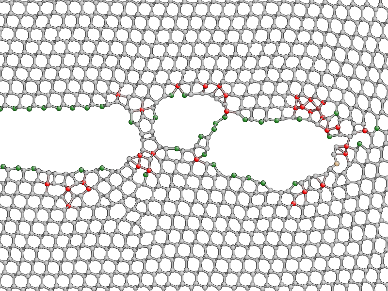
Geometry and coordination analysis

Press k to colour the atoms by coordination. This is based on the nneightol attribute of the Atoms object, which we set to a value of 1.3 in the make_crack.py script. This factor acts as a multipler for the covalent radii of the atomic species, taken from the quippy.periodictable.ElementCovRad array. You can check the maximum Si–Si bond-length this corresponds to with:

print 1.3*2*ElementCovRad[14]

Note that 14 is the atomic number of silicon. After the simulation has run for a little while, you should be able to see both under-coordinated (green) and over-coordinated (red) atoms near the crack tip.

Here is a typical snapshot at the end of 10 ps of dynamics. Note the large number of defects, indicating that the fracture surface is not atomically smooth as we find it to be in experiments. In your simulation you may be able to spot signs of energy dissipation mechanisms, such as dislocation emission from the crack tip.

Rendering a movie of the simulation

If you would like to make a movie of your simulation, you can use the render_movie() function. Arrange the AtomEye window so that the crack is on the left hand side of the window at the beginning of the simulation and near the right hand side at the end, then run the command:

render_movie('movie.mp4')

This function renders each frame to a .jpg file, before combining the snapshots with the ffmpeg tool to make a movie like this one:

The example movie above makes the ductile nature of the fracture propagation much clearer. We see local amorphisation, the formation of strange sp² tendrils, and temporary crack arrest. Comparing again with the experimental TEM images makes it clear that, as a description of fracture in real silicon, the SW potential falls some way short.

Position of the crack tip

The find_crack_tip_stress_field() function works by fitting per-atom stresses calculated with the SW potential (the concept of per-atom stresses will be discussed in more detail below) in the region near the crack tip to the Irwin solution for a singular crack tip under Mode I loading, which is of the form

\[\sigma_{ij}(r, \theta) = \frac{K_I}{2\pi r} f_{ij}(\theta)\]

where \(K_I\) is the Mode I stress intensity factor, and the angular dependence is given by the set of universal functions \(f_{ij}(\theta)\).

You can verify this by comparing the position detected by find_crack_tip_stress_field(), stored in the crack_pos attribute, with the positions of atoms that visually look to be near the tip — right click on atoms in the AtomEye viewer window to print information about them, including their positions.

Compare the automatically detected crack position (printed as the crack_pos_x parameter when you change frames in the AtomEye viewer, or available via gcat().info['crack_pos_x']) with what a visual inspection of the crack system would tell you. Do you think it’s accurate enough to use as the basis for selecting a region around the crack tip to be treated at the QM level?

Evolution of energy release rate and crack position

For netcdf trajectories, the AtomsReaderViewer.reader.netcdf_file attribute of the current viewer object gcv() provides direct access to the underlying NetCDF file using the Python netCDF4 module:

traj = gcv()
dataset = traj.reader.netcdf_file

You can list the variables stored in dataset with:

print dataset.variables.keys()

To plot the energy release rate G as a function of simulation time, you could do:

plot(dataset.variables['time'], dataset.variables['G'])

You should see that the energy release rate increases at a roughly constant rate before stopping at constant value when the crack starts to move (the increase is not linear since is is actually the strain that we increment at a constant rate).

The following plot shows the evolution of G (blue) and of the position of the crack (red; stored as crack_pos_x). Note that a second vertical axis can be produced with the twinx() function.

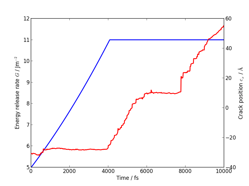
In this case the crack actually arrests for a while at around \(t = 6\) ps. This is another characteristic feature of non-brittle fracture, indicating that our simulation is failing to match well with experiment. According to Griffith’s criterion, fracture should initiate at \(2\gamma \sim 2.7\) J/m², whereas we don’t see any motion of the crack tip until \(G \sim 11\) J/m². How much of this difference do you think is due to the high strain rate and small system used here, and how much to the choice of interatomic potential? How would you check this?

Temperature and velocity analysis

Using the method above, plot the evolution of the temperature during your simulation. Here is another example plot, with the temperature shown in blue and the crack position in red.

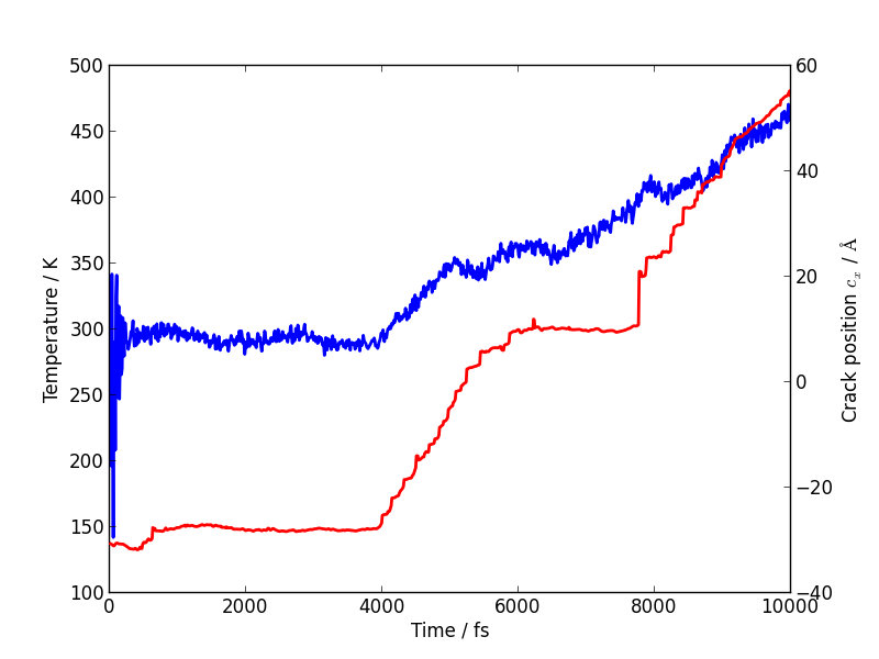
You will see that lots of heat is produced once the crack starts to move, indicating that the system is far from equilibrium. This is another sign that our system is rather small and our strain rate is rather high. How could this be addressed? Do you think an NVT simulation would be more realistic? What problems could adding a thermostat introduce?

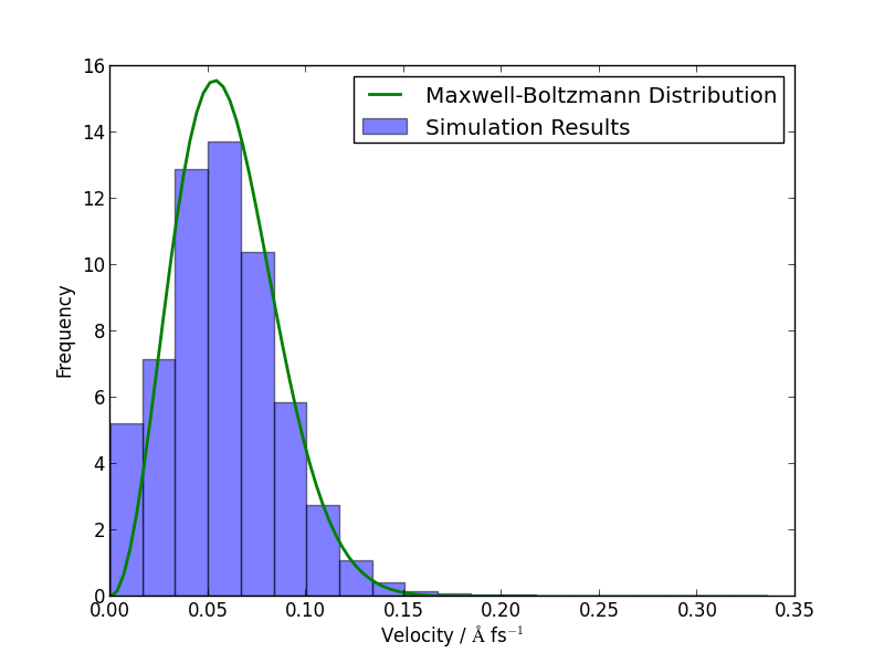
If you have time, you could compare how well the atomic velocities match the expected Maxwell-Boltzmann distribution of atomic velocities, given by

\[f(v)\,\mathrm{d}v = 4 \pi \left( \frac{m}{2 \pi k_B T} \right)^{3/2} v^2 \exp \left[ -\frac{mv^2}{2 k_B T} \right] \mathrm{d}v\]

Here’s a Python function which implements this formula:

def max_bolt(m,T,v):
   "Maxwell-Boltmann distribution of speeds at temperature T for particles of mass m"
   return 4*pi*(m/(2*pi*units.kB*T))**(3.0/2.0)*(v**2)*exp(-m*v**2/(2*units.kB*T))

We can average the atomic speeds in the last 50 frames in our trajectory and use the speeds data to produce a histogram:

m = traj[-1].get_masses()[0]      # Mass of a Si atom
T = traj[-1].info['temperature']  # Temperature at end of simulation
v = traj.reader.netcdf_file.variables['momenta'][-50:,:,:]/m # Get velocities
s = sqrt((v**2).sum(axis=2))      # Speeds are magnitude of velocities

hist(s.reshape(-1), 20, normed=True, alpha=0.5)  # Draw a histogram

ss = linspace(0., s.max(), 100)  # Compare with Maxwell-Boltzmann distrib
plot(ss, max_bolt(m,T,ss), lw=2)

Atom-resolved strain tensor

The virial stress expression above is only valid when averaged over time and space, so this method of calculating per-atom stresses can lead to unphysical oscillations [Zimmerman2004]. One alternative is the atom-resolved strain tensor, which allows the strain, and hence stress, fields to be evaluated at the atomistic scale facilitating direct comparisons with elasticity theory results [Moras2010].

A definition of the atom-resolved strain tensor can be obtained for all the four-fold coordinated atoms in the tetrahedral structure (all other atoms are assigned zero strain) by comparing the atomic positions with the unstrained crystal. The neighbours of each atom are used to define a local set of cubic axes, and the deformations along each of these axes are combined into a matrix \(E\) describing the local deformation:

\[\begin{split}E = \left(\begin{array}{ccc} | & | & | \\ \mathbf{e}_{1} & \mathbf{e}_{2} & \mathbf{e}_{3} \\ | & | & | \end{array}\right)\end{split}\]

where, for example \(\mathbf{e}_{1}\) is the relative deformation along the first cubic axis. To compute the local strain of the atom, we need to separate this deformation into a contribution due to rotation and one due to strain. This can be done by finding the polar decomposition of \(E\), by writing \(E\) in the form \(E = SR\) with \(R\) a pure rotation and \(S\) a symmetric matrix.

Diagonalising the product \(EE^T\) allows \(R\) and \(S\) to be calculated. The strain components \(\epsilon_{xx}\), \(\epsilon_{yy}\), \(\epsilon_{zz}\), \(\epsilon_{xy}\), \(\epsilon_{xz}\) and \(\epsilon_{yz}\) can then be calculated by rotating \(S\) to align the local cubic axes with the Cartesian axes:

\[\begin{split} R^T S R = I + \epsilon = \left(\begin{array}{ccc} 1 + \epsilon_{xx} & \frac{1}{2}\epsilon_{xy} & \frac{1}{2}\epsilon_{xz} \\ \frac{1}{2}\epsilon_{xy} & 1 + \epsilon_{yy} & \frac{1}{2}\epsilon_{yz} \\ \frac{1}{2}\epsilon_{xz} & \frac{1}{2}\epsilon_{yz} & 1 + \epsilon_{zz} \end{array}\right).\end{split}\]

Finally if we assume linear elasticity applies, the atomistic stress can be computed simply as \(\bm\sigma = C \bm\epsilon\) where \(C\) is the \(6\times6\) matrix of elastic constants.

The AtomResolvedStressField class implements this approach. To use it to calculate the stress in your crack_slab Atoms object, you can use the following code:

arsf = AtomResolvedStressField(bulk=si_bulk)
crack_slab.set_calculator(arsf)
ar_stress = crack_slab.get_stresses()

Colour your atoms by the \(\sigma_{yy}\) component of the atom-resolved stress field, and compare with the local virial stress results. Add the atom resolved \(\sigma_{yy}\) values along \(y = 0\) to your plot. Do you notice any significant differences? Repeat the minimisation of the crack slab with a lower value of relax_fmax (e.g. \(1 \times 10^{-3}\) eV/A). Do the stress components computed using the two methods change much?

When you are ready, proceed to Step 3: LOTF hybrid MD simulation of fracture in Si.