Step 3: LOTF hybrid MD simulation of fracture in Si
In the final part of this tutorial, we will be extending our previous script for classical molecular dynamics to carry out an adaptive QM/MM simulation of fracture using the ‘Learn on the Fly’ (LOTF) scheme.
You will need the run_crack_classical.py script from Step 2: Classical MD simulation of fracture in Si. If you
don’t have it, you can download it here,
and the crack.xyz input file from Step 1: Setup of the Silicon model system, which you
can also download here.
3.1 Initialisation of the QM/MM atomic system (20 minutes)
Import the relevant modules
Make a copy of your run_crack_classical.py script and name it
run_crack_lotf.py. Add the following extra import statements after those
that are already there:
from quippy.potential import ForceMixingPotential
from quippy.lotf import LOTFDynamics, update_hysteretic_qm_region
Definition of the simulation parameters
Next, we need to add some additional parameters specifically for the
QM/MM simulation. Again, insert them in run_crack_lotf.py, below the
existing parameters
qm_init_args = 'TB DFTB'         # Initialisation arguments for QM potential
qm_inner_radius = 8.0*units.Ang  # Inner hysteretic radius for QM region
qm_outer_radius = 10.0*units.Ang # Inner hysteretic radius for QM region
extrapolate_steps = 10           # Number of steps for predictor-corrector
                                 # interpolation and extrapolation
The setup of the atomic structure and of the constraints is exactly the same as before, so leave these sections of your script unchanged.
Setup of the QM and QM/MM potentials
For the QM/MM simulation, we first need to initialise the classical SW potential (mm_pot) and the quantum-mechanical one (qm_pot). The two Hamiltonians then need to be combined into a hybrid QM/MM potential (qmmm_pot), which mixes the QM and MM forces.
Leave the initialisiton of the SW classical potential as it is. After this, we
want to add some lines of code to setup the QM potential. Using the same
Potential class, we initialise now the Density
functional tight binding (DFTB) potential. This is done by passing the new QM
qm_init_args as the init_args parameter and the same XML file as before for
the param_filename to the Potential constructor (note that the single file
params.xml contains parameters for both the SW and DFTB potentials):
qm_pot = ... # Initialise DFTB potential
The QM/MM potential is constructed using quippy’s
quippy.potential.ForceMixingPotential class. Here, pot1 is
the low precision, i.e. MM potential, and pot2 is the high
precision, i.e. QM potential. fit_hops is the number of hops used to
define the fitting region, lotf_spring_hops defines the length of
the springs in the LOTF adjustable potential, while the hysteretic
buffer options control the size of the hysteretic buffer
region region used for the embedded QM force calculation.
qmmm_pot = ForceMixingPotential(pot1=mm_pot,
                                pot2=qm_pot,
        atoms=atoms,
                                qm_args_str='single_cluster cluster_periodic_z carve_cluster '+
                                            'terminate cluster_hopping=F randomise_buffer=F',
                                fit_hops=4,
                                lotf_spring_hops=3,
                                hysteretic_buffer=True,
                                hysteretic_buffer_inner_radius=7.0,
                                hysteretic_buffer_outer_radius=9.0,
                                cluster_hopping_nneighb_only=False,
                                min_images_only=True)
The qm_args_str argument defines some parameters which control how the QM calculation is carried out: we use a single cluster, periodic in the z direction and terminated with hydrogen atoms. The positions of the outer layer of buffer atoms are not randomised.
Change the line which sets the Atoms calculator to use the new qmmm_pot Potential:
atoms. ... # Set the calculator
Set up the initial QM region
Now, we can set up the list of atoms in the initial QM region using
the update_hysteretic_qm_region() function, defined
in quippy. Here we need to provide the Atoms system, the
centre of the QM region (i.e. the position of the crack tip), and the
the inner and outer radius of the hysteretic QM
region. Note that the old_qm_list attribute must be an empty list
([]) in this initial case:
qm_list = ... # Define the list of atoms in the QM region
The list needs to be attached to the qmmm_pot using the
set_qm_atoms() method:
qmmm_pot. ... # Attach QM list to calculator
Milestone 3.1
Your run_crack_lotf.py script should look something
like run_crack_lotf_1.py.
At this point you should run your script and check the initial QM region. For testing, you should add a couple of temporary lines to force the script to finish after setting the QM region and before repeating the classical MD:
import sys
sys.exit(0)
To visualise the initial QM region, you can type the following directly into
your ipython session (remember to do a from qlab import * first if you
haven’t already):
view(atoms)
aux_property_coloring(qmmm_pot.get_qm_atoms())
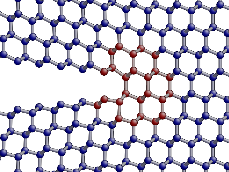
In the image above, the red atoms are QM and the blue atom classical.
Internally, this list is actually saved as a property inside the Atoms object named "hybrid",
which can also be displayed with aux_property_coloring("hybrid")
3.2 Setup and run the adaptive QM/MM MD (20 minutes)
Initialising the Dynamics
The definition of the initial temperature of the system should be left as in Step 2. Don’t forget to remove the temporary lines added above which quit the script after setting up the initial QM region!
Instead of a traditional dynamics in the NVE ensemble, let’s change the code to
use LOTF predictor-corrector dynamics, using
the quippy.lotf.LOTFDynamics class instead of
the VelocityVerlet class. We need to pass the following
arguments: atoms, timestep, extrapolate_steps (see Parameters
section):
dynamics = ... # Initialise the dynamical system
The logger and crack tip movement detection functions can be left almost exactly
as before for now: we just need to make a small change to
the printstatus() function so to distinguish between extrapolation and
interpolation:
Change the line:
atoms.info['label'] = 'D' # Label for the status line
to:
atoms.info['label'] = dynamics.state_label # Label for the status line
This uses the state_label attribute to print
an "E" at the beginning of the logger lines for extrapolation and an "I"
for interpolation.
Updating the QM region
We need to define a function that updates the QM region at the
beginning of each extrapolation cycle. As before, we need to find the
position of the crack tip and then update the hysteretic QM region. Note that now a previous QM region exists and
its atoms should be passed to the
update_hysteretic_qm_region() function. The current
QM atom list can be obtained with the
quippy.potential.ForceMixingPotential.get_qm_atoms() method. To
find the crack position, use
find_crack_tip_stress_field() as before, but pass
the MM potential as the calculator used to calculated the stresses
(force mixing potentials can only calculate forces, not per-atom
stresses; we will check later that the classical stress is
sufficiently accurate for locating the crack tip):
 def update_qm_region(atoms):
     crack_pos = ...          # Find crack tip position
     qm_list = ...            # Get current QM atoms
     qm_list = ...            # Update hysteretic QM region
     qmmm_pot. ...            # Set QM atoms

dynamics.set_qm_update_func(update_qm_region)
Writing the trajectory
Finally, we want to save frames to the trajectory every traj_interval time
steps but, this time, only during the interpolation phase of the
predictor-corrector cycle. To do this, we first initialise the trajectory file
(see AtomsWriter()), and then define a function that only
writes to the trajectory file if the state of the dynamical systems is
Interpolation:
trajectory = ... # Initialise trajectory using traj_file

def traj_writer(dynamics):
    if dynamics.state == LOTFDynamics.Interpolation:
        trajectory.write(dynamics.atoms)
As before, we attach this function to the dynamical system, passing
traj_interval and and extra argument of dynamics which gets passed along to the
traj_writer function (see the attach()
method):
dynamics. ... # Attach traj_writer to dynamics
Now, we can simply run the dynamics for nsteps steps:
dynamics. ... # Run dynamics for nsteps
If you are interested in seeing how the LOTF predictor-corrector cycle is
implemented, look at the documentation and source code for the
quippy.lotf.LOTFDynamics.step() routine.
Milestone 3.2
The finished version of the run_crack_lotf.py script should look something
like Step 3 solution — run_crack_lotf.py. To clearly show the differences with respect to the
classical MD script, here is a patch which could be used to convert the classical
script into the LOTF one.
3.3 Visualisation and Analysis (as time permits)
Predictor/corrector dynamics output file
Let’s first take a moment to look at the output of the script for the first predictor/corrector cycle. Here we go through some example output, yours should be similar. First there are a few lines about the initialisation of the system, and then we get the results of the initial LOTF adjustable potential optimisation:
Loading atoms from file crack.xyz
Fixed 240 atoms

25 atoms selected for quantum treatment
update_qm_region: QM region with 25 atoms centred on [-30.60517303   0.08401087   0.        ]
Adding default springs
Got 1484 springs
Number of force components: 297
Number of parameters:       1484
Optimising 1484 adjustable parameters
RMS force component error before optimisation : .05630875465645784
Max force component error before optimisation : .34841292159055509
Using SVD for least squares fit, eigenvalue threshold = .00000000010000000
RMS force component error after  optimisation :   0.27E-02
Max force component error after  optimisation :   0.61E-02
Max abs spring constant   after  optimisation :   0.45E-01
You can see that before adjusting the parameters, the QM and classical potentials differed by a maximum of 0.35 eV/A, with an RMS difference of 0.06 eV/A - in this case the SW potential is actually doing a rather respectable job. After the fit, which is this case involved 1484 spring parameters to fit 297 force component, the force differences are of course much smaller.
Next we start the first predictor/corrector cycle. First we update the QM region, and remap the adjustable potential to take account of any changes since last time:
25 atoms selected for quantum treatment
update_qm_region: QM region with 25 atoms centred on [-30.6048418    0.08377744   0.        ]
Adding default springs
Got 1484 springs
Number of force components: 297
Number of parameters:       1484
As this is the first step, there were no changes, so no re-optimisation is required. Next we carry out 10 steps of extrapolation, with constant LOTF adjustable parameters. During this time the strain is incremented as normal:
State      Time/fs    Temp/K     Strain      G/(J/m^2)  CrackPos/A D(CrackPos)/A
---------------------------------------------------------------------------------
E            1.0  553.716406     0.08427      5.0012      -30.61    (-0.00)
E            2.0  547.749233     0.08428      5.0024      -30.61    (-0.01)
E            3.0  535.952151     0.08429      5.0036      -30.62    (-0.01)
E            4.0  518.731103     0.08430      5.0047      -30.63    (-0.02)
E            5.0  496.675925     0.08431      5.0059      -30.63    (-0.03)
E            6.0  470.538607     0.08432      5.0071      -30.64    (-0.04)
E            7.0  441.205418     0.08433      5.0083      -30.65    (-0.05)
E            8.0  409.663780     0.08434      5.0095      -30.66    (-0.06)
E            9.0  376.965040     0.08435      5.0107      -30.67    (-0.07)
E           10.0  344.184506     0.08436      5.0119      -30.69    (-0.08)
At the end of the extrapolation, it’s time for a QM force evaluation and another fit. Now the force errors before fitting are a little larger, but the fit is still very good:
Optimising 1484 adjustable parameters
RMS force component error before optimisation : .10494977522791650
Max force component error before optimisation : .48515966905523733
Using SVD for least squares fit, eigenvalue threshold = .00000000010000000
RMS force component error after  optimisation :   0.37E-02
Max force component error after  optimisation :   0.96E-02
Max abs spring constant   after  optimisation :   0.83E-01
We next return to the initial dynamical state and re-run the dynamics, interpolating between the optimised parameters at the two ends of the cycle. Note that the strain is also returned to the initial value at \(t = 0\), and that the temperature after one step exactly matches the interpolation phase (since the forces and velocities at \(t = 0\) are identical for extrapolation and interpolation):
State      Time/fs    Temp/K     Strain      G/(J/m^2)  CrackPos/A D(CrackPos)/A
---------------------------------------------------------------------------------
I            1.0  553.716406     0.08427      5.0012      -30.65    (-0.04)
I            2.0  547.759567     0.08428      5.0024      -30.65    (-0.05)
I            3.0  535.982832     0.08429      5.0036      -30.66    (-0.05)
I            4.0  518.791314     0.08430      5.0047      -30.66    (-0.06)
I            5.0  496.773542     0.08431      5.0059      -30.67    (-0.07)
I            6.0  470.679783     0.08432      5.0071      -30.68    (-0.08)
I            7.0  441.394231     0.08433      5.0083      -30.69    (-0.09)
I            8.0  409.901969     0.08434      5.0095      -30.70    (-0.10)
I            9.0  377.251837     0.08435      5.0107      -30.71    (-0.11)
I           10.0  344.516566     0.08436      5.0119      -30.73    (-0.12)
To continue from here, we simply go back to the extrapolation phase and then repeat the entire cycle.
QM active and buffer regions
Trajectory analysis
Open your new trajectory as before, using the
view() function from within a new ipython session, and
visualise the QM region by colouring the atoms using the
hybrid_mark property
aux_property_coloring("hybrid_mark")
This property is used internally to identify which atoms are used for the QM active and buffer regions:
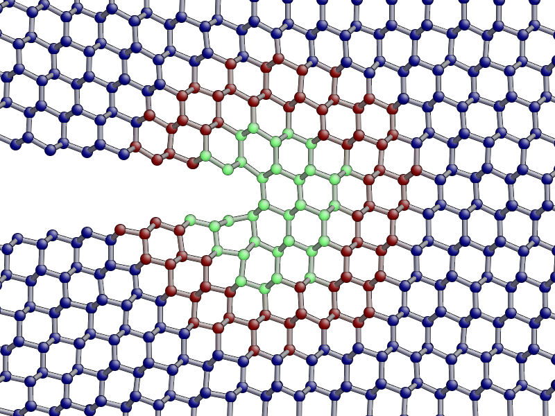
The central green atoms have hybrid_mark == HYBRID_ACTIVE_MARK, and they are
the atoms for which QM forces are used to propagate the dynamics. Classical
forces are used for all other atoms, including the red buffer region, where
hybrid_mark == HYBRID_BUFFER_MARK. As explained above, the
purpose of the buffer region is to give accurate QM forces on the active atoms.
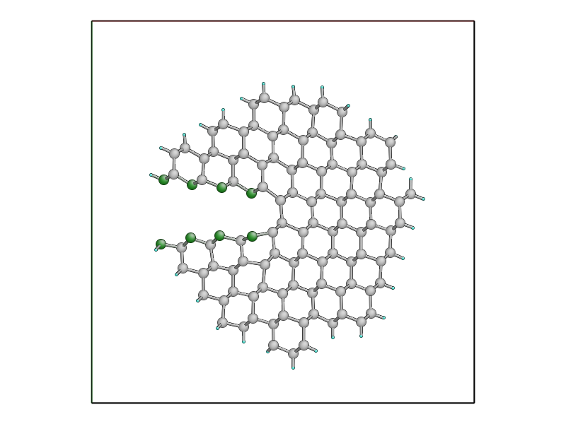
If you want to see the actual cluster used for carrying out the embedded DFTB
calculation, you could use the create_cluster_simple()
function together with the same args_str cluster options defined above:
cluster = create_cluster_simple(gcat(),
               args_str=("single_cluster cluster_periodic_z carve_cluster "
                         "terminate cluster_hopping=F randomise_buffer=F"))
view(cluster)
Colouring the cluster by coordination (press k) can be useful to check that all cut bonds have been correctly passivated by hydrogen atoms:
Comparison between classical and LOTF dynamics
Step through your trajectory with the Insert and Delete keys to see what happens in the LOTF dynamics. As before, you can jump to the end with Ctrl+Delete. You should find that the dynamics is very different to the classical case.
Check if the QM region is following the moving crack properly by looking at the
hybrid_mark property. If you repeat the analysis of the stress field carried out in Step 2, you should find that
the time averaged stress field is strongly concentrated
on the sharp crack tip. It is this stress field which is used
by find_crack_tip_stress_field() to follow the crack tip,
and hence to update the set of atoms in the QM region.
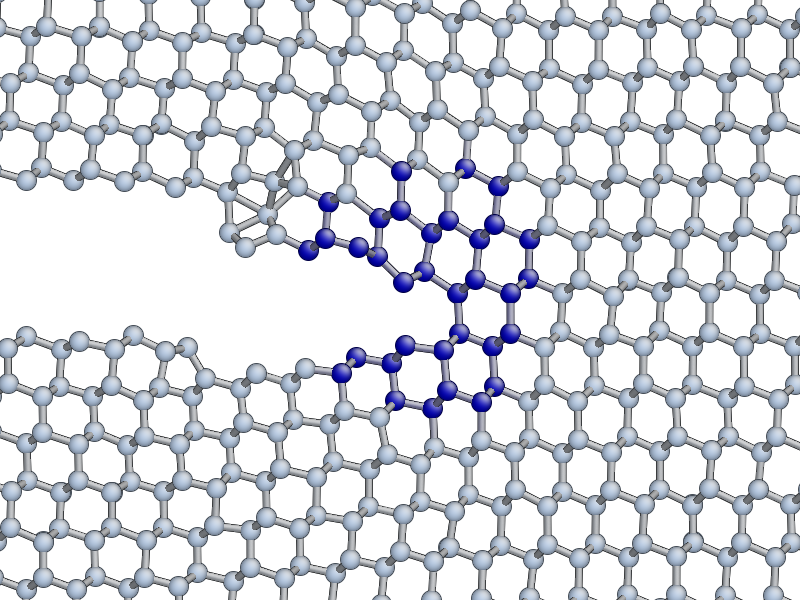
Here is a movie of a typical LOTF simulation on the \((111)\) cleavage
plane. To colour the QM atoms dark blue, we passed
the highlight_qm_region() function as the hook argument
to render_movie():
During the LOTF dynamics, the time-averaged stress field smoothly tracks the crack tip, as can be seen in this movie, where atoms are coloured by their \(\sigma_{yy}\) component:
And here is a head-to-head comparison of SW and LOTF dynamics:
Fracture initiates much earlier in the LOTF case, i.e. at a much reduced energy release rate, and is much more brittle, with none of the artificial plasticity seen with the classical potential alone.
Note that if you continue the LOTF dynamics, however, we may see some defects in the frature surface after the crack has propagated for a few nm. These are associated with the relatively small system and high strain rate we are using here, which leads to fracture at high energies and possibly to high speed fracture instabilities [Fineberg1991]. If you have time you can investigate this in the extension task on size and strain rate effects.
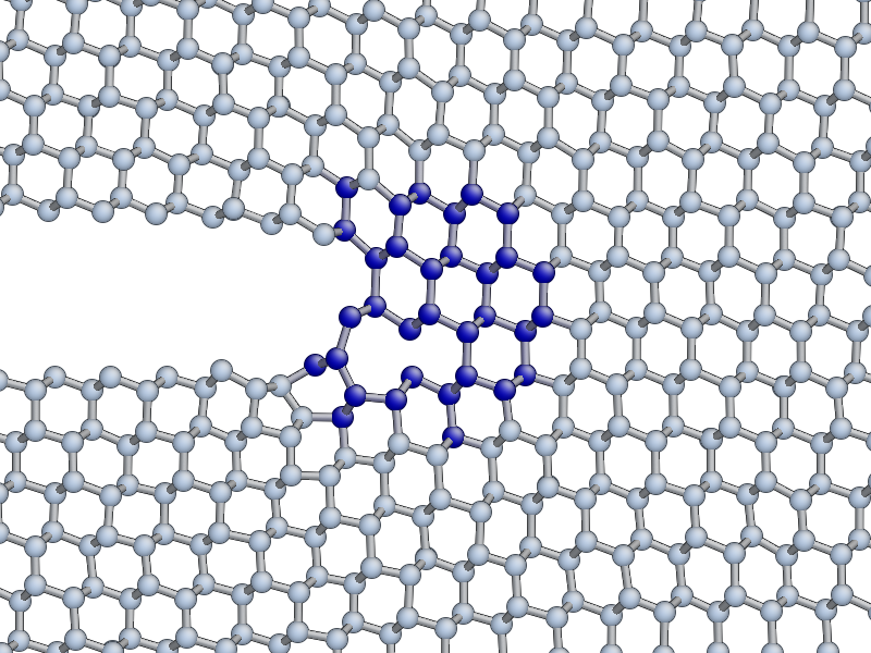
Although it is beyond the scope of this tutorial, you might be interested to know that using an overall larger system, bigger QM region and lower strain rate, as well as changing the Hamiltonian from DFTB to DFT-GGA, removes all of these defects, recovering perfectly brittle fracture propagation. The DFT model also gives an improved description of the fracture surfaces, which reconstruct to form a Pandey \(\pi\)-bonded chain, with it’s characteristic alternating pentagons and heptagons:
Evolution of energy release rate and crack position
If you follow the previous approach to plot the energy release rate G and crack position crack_pos_x variables during your LOTF simulation, you should find that the crack now advances monotonically, with a constant crack velocity of around 2500 m/s, and at about half the energy release rate of the classical case (6 J/m2 vs 12 J/m2).
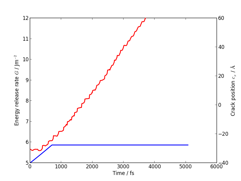
For comparison, here is the classical plot again:
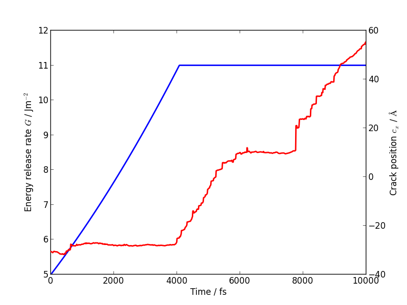
You should find that the temperature still goes up, but more gently than in the classical case, since the flow of energy to the crack tip is closer to the energy consumed by creating the new surfaces. Some heat is generated at the QM/MM border; usually this would be controlled with a gentle Langevin thermostat, which we have omitted here in the interests of simplicity.
Low speed instability on the (111) cleavage plane
If you are lucky, you may see the formation of a crack tip reconstruction consisting of a 5 and a 7 membered ring on the lower fracture surface, related to the Pandey surface reconstruction.
This reconstruction can cause cracks to take a step down by one atomic layer, which over time can build up via positive feedback mechanism into an experimentally observable phenomena [Kermode2008].
3.4 Checking the predictor/corrector force errors (optional)
Add check_force_error=True to the LOTFDynamics
constructor. This causes the LOTF routines to do a reference QM force evaluation
at every timestep (note that these extra QM forces are not used in the fitting,
so the dynamical trajectory followed is the same as before).
When checking the predictor/corrector errors, you need to disable the updating of the QM region by commenting out the line:
dynamics.set_qm_update_func(update_qm_region)
Let’s create a logfile to save the force errors at each step during
the interpolation and extrapolation. Add the following code before the
dynamics.run() call:
def log_pred_corr_errors(dynamics, logfile):
    logfile.write('%s err %10.1f%12.6f%12.6f\n' % (dynamics.state_label,
                                                   dynamics.get_time()/units.fs,
                                                   dynamics.rms_force_error,
                                                   dynamics.max_force_error))
logfile = open('pred-corr-error.txt', 'w')
dynamics.attach(log_pred_corr_errors, 1, dynamics, logfile)
Finally, change the total number of steps (via the nsteps parameter) to a much
smaller number (e.g. 200 steps), close the logfile after the dynamics.run()
line:
logfile.close()
Once the dynamics have run for a few LOTF cycles, you can plot the results with
a shell script called plot_pred_corr_errors.py:
plot_pred_corr_errors.py -e 10 pred-corr-error.txt
The -e 10 argument is used to specify the number of extrapolate steps. This
produces a set of four plots giving the RMS and maximum force errors during
extrapolation and interpolation:
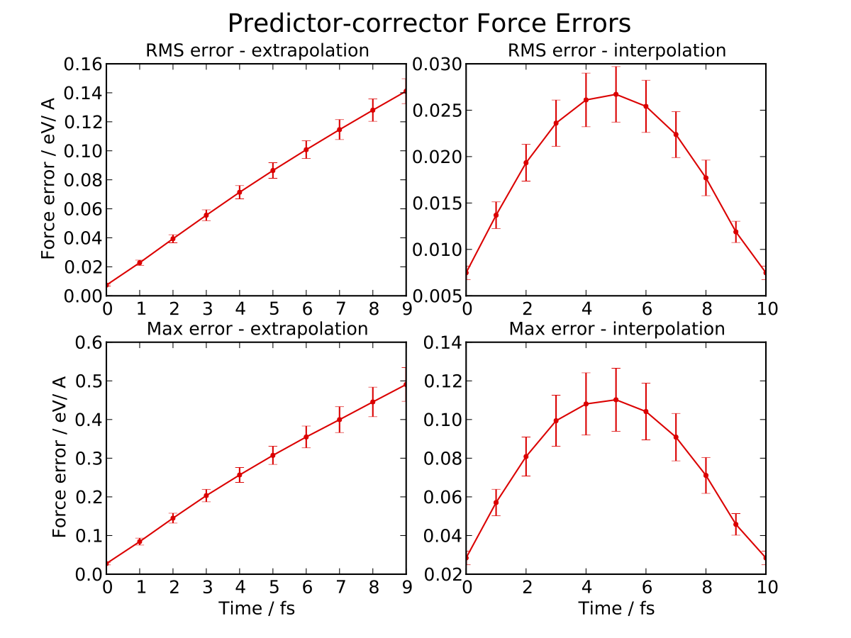
Note that the scale is different on the extrapolation and interpolation plots! Try varying the extrapolate_steps parameter and seeing what the effect on force errors is. What is the largest acceptable value? You could also try changing the lotf_spring_hops and fit_hops parameters, which control the maximum length of the corrective springs added to the potential and the size of the fit region, respectively.
Milestone 3.4
Here is a final version of the run_crack_lotf.py script including
checking of the force errors: run_crack_lotf.py.
Further extension tasks
QM region size
Investigate the effect of increasing the QM region size, controlled by the qm_inner_radius and qm_outer_radius parameters. When does the behaviour converge qualitatively? What does this say about the size of the ‘process zone’ in silicon?
Buffer region size
We have used a hysteretic buffer region from 7 A to 9 A. How would you check if this is sufficient? What criteria need to be satisfied for our results to be considered to be converged with respect to buffer region size?
Crack energy-speed relationship
Try varying the flow of energy to the crack tip by changing the initial_G parameter used when making the crack system in Step 1: Setup of the Silicon model system. How does this affect the speed of the crack?
Other crack orientations
Return to the beginning of Step 1: Setup of the Silicon model system and try classical and/or LOTF dynamics (which will actually probably be faster!) on the \((110)\) surface. Do you see any major differences? Can you find any dynamic fracture instabilities?
System size and strain rate effects
What is the effect of changing the system size on the critical energy release rate for fracture? How would you converge with respect to this parameter? Do you think experimental length scales can be reached? If not, does it matter? Think about how the choice of loading geometry helps here.
As well as finite size effects, and perhaps more severely, we are limited in the time scales that can be accessed by our fracture simulations, especially when using a QM method to describe the crack tip processes. Are there any scaling relations that can help us out here? How would you estimate the effect of the artificially high strain rate we have been forced to impose here.