Poisson-Nernst-Planck systems by finite element method

PoissonNernstPlanckSystem of matscipy.electrochemistry.poisson_nernst_planck_solver uses its own controlled-volumes solver implementation, while PoissonNernstPlanckSystemFEniCS of matscipy.electrochemistry.poisson_nernst_planck_solver_fenics interfaces the finite elements solver FEniCS for solving Poisson-Nernst-Planck systems. In highly nonlinear problems, latter may offer improved convergence above the former. Following examples illustrate this.

Again, we look at the inert electrode shown here.

Figure 1: Inert electrode at the open half-space

As usual, we begin with preparing a few necessities.

# basics
import numpy as np
import scipy.constants as sc
import matplotlib.pyplot as plt

# electrochemistry basics
from matscipy.electrochemistry import debye, ionic_strength

# Poisson-Bolzmann distribution
from matscipy.electrochemistry.poisson_boltzmann_distribution import gamma, potential, concentration, charge_density

# Poisson-Nernst-Planck solver
from matscipy.electrochemistry import PoissonNernstPlanckSystem
from matscipy.electrochemistry.poisson_nernst_planck_solver_fenics import PoissonNernstPlanckSystemFEniCS

# 3rd party file output
import ase
import ase.io

def make_patch_spines_invisible(ax):
    ax.set_frame_on(True)
    ax.patch.set_visible(False)
    for sp in ax.spines.values():
        sp.set_visible(False)

pnp = {}

/usr/lib/python3/dist-packages/scipy/__init__.py:146: UserWarning: A NumPy version >=1.17.3 and <1.25.0 is required for this version of SciPy (detected version 1.26.4
  warnings.warn(f"A NumPy version >={np_minversion} and <{np_maxversion}"

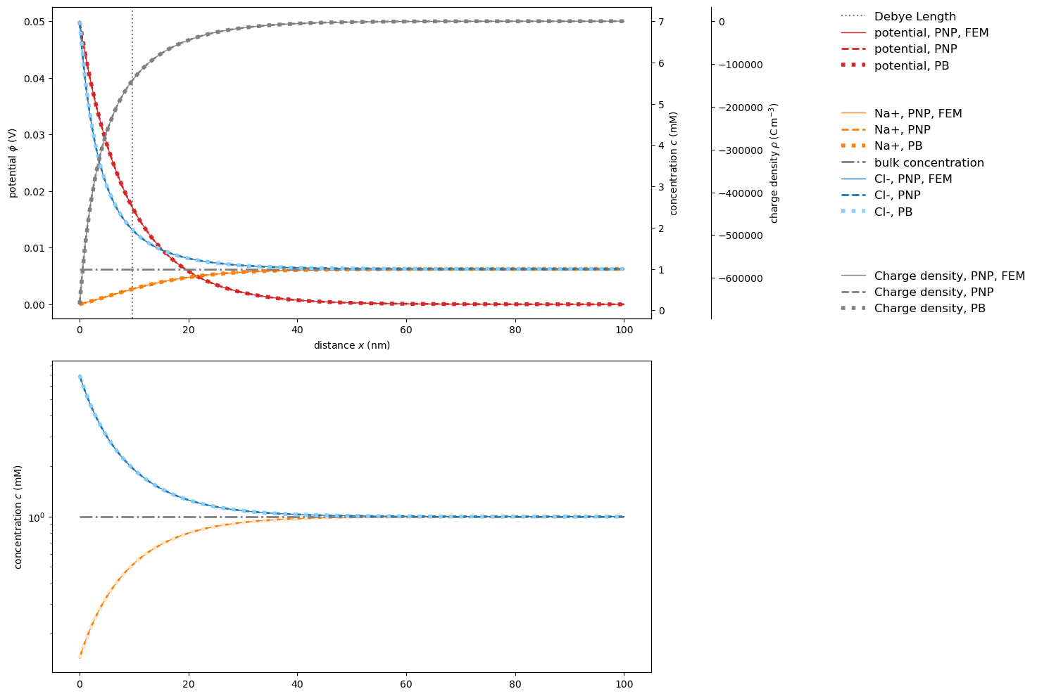
Agreement of solvers for moderate boundary conditions

At moderate potentials across the interface, both PoissonNernstPlanckSystem and PoissonNernstPlanckSystemFEniCS both converge quickly.

# Test case parameters
c = [1.0, 1.0]
z = [1, -1]
L = 100e-9 # 100 nm
delta_u = 0.05 # V
N = 200 # number of discretization grid points

# define desired system
pnp['std_interface'] = PoissonNernstPlanckSystem(
    c, z, L, delta_u=delta_u, N=N,
    solver="hybr", options={'xtol':1e-12})

pnp['std_interface'].use_standard_interface_bc()
uij, nij, lamj = pnp['std_interface'].solve()

# define desired system
pnp['fenics_interface'] = PoissonNernstPlanckSystemFEniCS(c, z, L, delta_u=delta_u, N=N)
pnp['fenics_interface'].use_standard_interface_bc()
uij, nij, _ = pnp['fenics_interface'].solve()

/usr/lib/python3/dist-packages/scipy/optimize/_root.py:208: RuntimeWarning: Method hybr does not accept callback.
  warn('Method %s does not accept callback.' % method,

Calling FFC just-in-time (JIT) compiler, this may take some time.

Calling FFC just-in-time (JIT) compiler, this may take some time.

Calling FFC just-in-time (JIT) compiler, this may take some time.

Calling FFC just-in-time (JIT) compiler, this may take some time.
No Jacobian form specified for nonlinear variational problem.
Differentiating residual form F to obtain Jacobian J = F'.

Calling FFC just-in-time (JIT) compiler, this may take some time.

Calling FFC just-in-time (JIT) compiler, this may take some time.

Calling FFC just-in-time (JIT) compiler, this may take some time.

Solving nonlinear variational problem.
  Newton iteration 0: r (abs) = 2.287e+02 (tol = 1.000e-10) r (rel) = 1.000e+00 (tol = 1.000e-09)
  Newton iteration 1: r (abs) = 2.656e-01 (tol = 1.000e-10) r (rel) = 1.161e-03 (tol = 1.000e-09)
  Newton iteration 2: r (abs) = 5.172e+00 (tol = 1.000e-10) r (rel) = 2.262e-02 (tol = 1.000e-09)
  Newton iteration 3: r (abs) = 9.975e-01 (tol = 1.000e-10) r (rel) = 4.362e-03 (tol = 1.000e-09)
  Newton iteration 4: r (abs) = 6.783e-04 (tol = 1.000e-10) r (rel) = 2.966e-06 (tol = 1.000e-09)
  Newton iteration 5: r (abs) = 9.937e-12 (tol = 1.000e-10) r (rel) = 4.345e-14 (tol = 1.000e-09)
  Newton solver finished in 5 iterations and 5 linear solver iterations.

The results fall onto each other and onto the analytical Poisson-Boltzmann solution, validating each other.

x = np.linspace(0,L,100)
phi = potential(x, c, z, delta_u) 
C =   concentration(x, c, z, delta_u)
rho = charge_density(x, c, z, delta_u) 
deb = debye(c, z)

fig, (ax1, ax4) = plt.subplots(nrows=2, ncols=1, figsize=[16, 10])

ax1.axvline(x=deb/sc.nano, label='Debye Length', color='grey', linestyle=':')

ax1.plot(
    pnp['fenics_interface'].grid/sc.nano, pnp['fenics_interface'].potential, 
    marker='', color='tab:red', label='potential, PNP, FEM', linewidth=1, linestyle='-')
ax1.plot(
    pnp['std_interface'].grid/sc.nano, pnp['std_interface'].potential, 
    marker='', color='tab:red', label='potential, PNP', linewidth=2, linestyle='--')
ax1.plot(
    x/sc.nano, phi, 
    marker='', color='tab:red', label='potential, PB', linewidth=4, linestyle=':')

ax2 = ax1.twinx()
ax2.plot(pnp['fenics_interface'].grid/sc.nano, pnp['fenics_interface'].concentration[0], 
    marker='', color='tab:orange', label='Na+, PNP, FEM', linewidth=1, linestyle='-')
ax2.plot(pnp['std_interface'].grid/sc.nano, pnp['std_interface'].concentration[0], 
    marker='', color='tab:orange', label='Na+, PNP', linewidth=2, linestyle='--')
ax2.plot(x/sc.nano, C[0], 
    marker='', color='tab:orange', label='Na+, PB', linewidth=4, linestyle=':')
ax2.plot(x/sc.nano, np.ones(x.shape)*c[0], 
    label='bulk concentration', color='grey', linewidth=2, linestyle='-.')


ax2.plot(pnp['fenics_interface'].grid/sc.nano, pnp['fenics_interface'].concentration[1], 
    marker='', color='tab:blue', label='Cl-, PNP, FEM', linewidth=1, linestyle='-')
ax2.plot(pnp['std_interface'].grid/sc.nano, pnp['std_interface'].concentration[1], 
    marker='', color='tab:blue', label='Cl-, PNP', linewidth=2, linestyle='--')
ax2.plot(x/sc.nano, C[1], 
    marker='', color='lightskyblue', label='Cl-, PB', linewidth=4, linestyle=':')


ax3 = ax1.twinx()
# Offset the right spine of ax3.  The ticks and label have already been
# placed on the right by twinx above.
ax3.spines["right"].set_position(("axes", 1.1))
# Having been created by twinx, ax3 has its frame off, so the line of its
# detached spine is invisible.  First, activate the frame but make the patch
# and spines invisible.
make_patch_spines_invisible(ax3)
# Second, show the right spine.
ax3.spines["right"].set_visible(True)

ax3.plot(pnp['fenics_interface'].grid/sc.nano, pnp['fenics_interface'].charge_density, 
    label='Charge density, PNP, FEM', color='grey', linewidth=1, linestyle='-')
ax3.plot(pnp['std_interface'].grid/sc.nano, pnp['std_interface'].charge_density, 
    label='Charge density, PNP', color='grey', linewidth=2, linestyle='--')
ax3.plot(x/sc.nano, rho, 
    label='Charge density, PB', color='grey', linewidth=4, linestyle=':')

ax4.semilogy(
    pnp['fenics_interface'].grid/sc.nano, 
    pnp['fenics_interface'].concentration[0], marker='', color='tab:orange', 
    label='Na+, PNP, FEM', linewidth=1, linestyle='-')
ax4.semilogy(
    pnp['std_interface'].grid/sc.nano, 
    pnp['std_interface'].concentration[0], marker='', color='tab:orange', 
    label='Na+, PNP', linewidth=2, linestyle='--')
ax4.semilogy(x/sc.nano, C[0], 
    marker='', color='bisque', label='Na+, PB', linewidth=4, linestyle=':')
ax4.semilogy(x/sc.nano, np.ones(x.shape)*c[0], 
    label='bulk concentration', color='grey', linewidth=2, linestyle='-.')

ax4.semilogy(
    pnp['fenics_interface'].grid/sc.nano, pnp['fenics_interface'].concentration[1], 
    marker='', color='tab:blue', label='Cl-, PNP, FEM', linewidth=1, linestyle='-')
ax4.semilogy(
    pnp['std_interface'].grid/sc.nano, pnp['std_interface'].concentration[1], 
    marker='', color='tab:blue', label='Cl-, PNP', linewidth=2, linestyle='--')
ax4.semilogy(x/sc.nano, C[1], 
    marker='', color='lightskyblue', label='Cl-, PB',linewidth=4,linestyle=':')

ax1.set_xlabel('distance $x$ (nm)')
ax1.set_ylabel('potential $\phi$ (V)')
ax2.set_ylabel('concentration $c$ (mM)')
ax3.set_ylabel(r'charge density $\rho \> (\mathrm{C}\> \mathrm{m}^{-3})$')
ax4.set_ylabel('concentration $c$ (mM)')

ax1.legend(loc='upper left',  bbox_to_anchor=(1.3,1.02), fontsize=12, frameon=False)
ax2.legend(loc='center left', bbox_to_anchor=(1.3,0.5),  fontsize=12, frameon=False)
ax3.legend(loc='lower left',  bbox_to_anchor=(1.3,-0.02), fontsize=12, frameon=False)

fig.tight_layout()
plt.show()

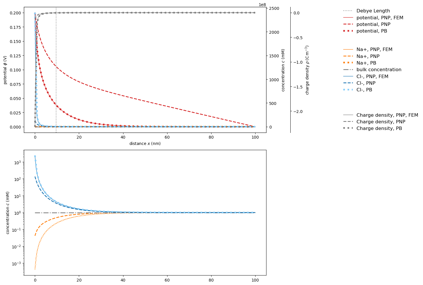
Convergence issues for extreme nonlinearities

At boundary conditions leading to extremely nonlinear behavior close to the interface, the third-party finite elements solver outperforms our controlled-volumes solver.

# Test case parameters   oö
c = [1.0, 1.0]
z = [1, -1]
L = 100e-9 # 100 nm
delta_u = 0.2 # V
N = 200

pnp['std_interface_high_potential'] = PoissonNernstPlanckSystem(
    c, z, L, delta_u=delta_u,N=N,
    solver="hybr", options={'xtol':1e-14})
pnp['std_interface_high_potential'].use_standard_interface_bc()
uij, nij, lamj = pnp['std_interface_high_potential'].solve()

/usr/lib/python3/dist-packages/scipy/optimize/_root.py:208: RuntimeWarning: Method hybr does not accept callback.
  warn('Method %s does not accept callback.' % method,

The iteration is not making good progress, as measured by the 
  improvement from the last ten iterations.

Apparently, the PoissonNernstPlanckSystem controlled-volumes solver does not converge …

pnp['fenics_interface_high_potential'] = PoissonNernstPlanckSystemFEniCS(c, z, L, delta_u=delta_u, N=200)
pnp['fenics_interface_high_potential'].use_standard_interface_bc()
uij, nij, _ = pnp['fenics_interface_high_potential'].solve()

No Jacobian form specified for nonlinear variational problem.
Differentiating residual form F to obtain Jacobian J = F'.
Solving nonlinear variational problem.
  Newton iteration 0: r (abs) = 7.521e+02 (tol = 1.000e-10) r (rel) = 1.000e+00 (tol = 1.000e-09)
  Newton iteration 1: r (abs) = 1.062e+00 (tol = 1.000e-10) r (rel) = 1.413e-03 (tol = 1.000e-09)
  Newton iteration 2: r (abs) = 1.796e+02 (tol = 1.000e-10) r (rel) = 2.388e-01 (tol = 1.000e-09)
  Newton iteration 3: r (abs) = 8.177e+03 (tol = 1.000e-10) r (rel) = 1.087e+01 (tol = 1.000e-09)
  Newton iteration 4: r (abs) = 2.132e+04 (tol = 1.000e-10) r (rel) = 2.834e+01 (tol = 1.000e-09)
  Newton iteration 5: r (abs) = 9.154e+02 (tol = 1.000e-10) r (rel) = 1.217e+00 (tol = 1.000e-09)
  Newton iteration 6: r (abs) = 3.454e-02 (tol = 1.000e-10) r (rel) = 4.592e-05 (tol = 1.000e-09)
  Newton iteration 7: r (abs) = 1.724e-10 (tol = 1.000e-10) r (rel) = 2.292e-13 (tol = 1.000e-09)
  Newton solver finished in 7 iterations and 7 linear solver iterations.

… while PoissonNernstPlanckSystemFEniCS does. Visualizing the results proves the agreement of finite elements results and analytical solution.

x = np.linspace(0, L, 100)
phi = potential(x, c, z, delta_u) 
C =   concentration(x, c, z, delta_u)
rho = charge_density(x, c, z, delta_u) 
deb = debye(c, z)

fig, (ax1, ax4) = plt.subplots(nrows=2, ncols=1, figsize=[16, 10])

ax1.axvline(x=deb/sc.nano, label='Debye Length', color='grey', linestyle=':')

ax1.plot(
    pnp['fenics_interface_high_potential'].grid/sc.nano, pnp['fenics_interface_high_potential'].potential, 
    marker='', color='tab:red', label='potential, PNP, FEM', linewidth=1, linestyle='-')
ax1.plot(
    pnp['std_interface_high_potential'].grid/sc.nano, pnp['std_interface_high_potential'].potential, 
    marker='', color='tab:red', label='potential, PNP', linewidth=2, linestyle='--')
ax1.plot(
    x/sc.nano, phi, 
    marker='', color='tab:red', label='potential, PB', linewidth=4, linestyle=':')


ax2 = ax1.twinx()
ax2.plot(pnp['fenics_interface_high_potential'].grid/sc.nano, pnp['fenics_interface_high_potential'].concentration[0], 
    marker='', color='tab:orange', label='Na+, PNP, FEM', linewidth=1, linestyle='-')
ax2.plot(pnp['std_interface_high_potential'].grid/sc.nano, pnp['std_interface_high_potential'].concentration[0], 
    marker='', color='tab:orange', label='Na+, PNP', linewidth=2, linestyle='--')
ax2.plot(x/sc.nano, C[0], 
    marker='', color='tab:orange', label='Na+, PB', linewidth=4, linestyle=':')
ax2.plot(x/sc.nano, np.ones(x.shape)*c[0], 
    label='bulk concentration', color='grey', linewidth=2, linestyle='-.')


ax2.plot(pnp['fenics_interface_high_potential'].grid/sc.nano, pnp['fenics_interface_high_potential'].concentration[1], 
    marker='', color='tab:blue', label='Cl-, PNP, FEM', linewidth=1, linestyle='-')
ax2.plot(pnp['std_interface_high_potential'].grid/sc.nano, pnp['std_interface_high_potential'].concentration[1], 
    marker='', color='tab:blue', label='Cl-, PNP', linewidth=2, linestyle='--')
ax2.plot(x/sc.nano, C[1], 
    marker='', color='lightskyblue', label='Cl-, PB', linewidth=4, linestyle=':')


ax3 = ax1.twinx()
# Offset the right spine of ax3.  The ticks and label have already been
# placed on the right by twinx above.
ax3.spines["right"].set_position(("axes", 1.1))
# Having been created by twinx, ax3 has its frame off, so the line of its
# detached spine is invisible.  First, activate the frame but make the patch
# and spines invisible.
make_patch_spines_invisible(ax3)
# Second, show the right spine.
ax3.spines["right"].set_visible(True)

ax3.plot(pnp['fenics_interface_high_potential'].grid/sc.nano, pnp['fenics_interface_high_potential'].charge_density, 
    label='Charge density, PNP, FEM', color='grey', linewidth=1, linestyle='-')
ax3.plot(pnp['std_interface_high_potential'].grid/sc.nano, pnp['std_interface_high_potential'].charge_density, 
    label='Charge density, PNP', color='grey', linewidth=2, linestyle='--')
ax3.plot(x/sc.nano, rho, 
    label='Charge density, PB', color='grey', linewidth=4, linestyle=':')


ax4.semilogy(
    pnp['fenics_interface_high_potential'].grid/sc.nano, 
    pnp['fenics_interface_high_potential'].concentration[0], marker='', color='tab:orange', 
    label='Na+, PNP, FEM', linewidth=1, linestyle='-')
ax4.semilogy(
    pnp['std_interface_high_potential'].grid/sc.nano, 
    pnp['std_interface_high_potential'].concentration[0], marker='', color='tab:orange', 
    label='Na+, PNP', linewidth=2, linestyle='--')
ax4.semilogy(x/sc.nano, C[0], 
    marker='', color='bisque', label='Na+, PB', linewidth=4, linestyle=':')
ax4.semilogy(x/sc.nano, np.ones(x.shape)*c[0], 
    label='bulk concentration', color='grey', linewidth=2, linestyle='-.')


ax4.semilogy(
    pnp['fenics_interface_high_potential'].grid/sc.nano, pnp['fenics_interface_high_potential'].concentration[1], 
    marker='', color='tab:blue', label='Cl-, PNP, FEM', linewidth=1, linestyle='-')
ax4.semilogy(
    pnp['std_interface_high_potential'].grid/sc.nano, pnp['std_interface_high_potential'].concentration[1], 
    marker='', color='tab:blue', label='Cl-, PNP', linewidth=2, linestyle='--')
ax4.semilogy(x/sc.nano, C[1], 
    marker='', color='lightskyblue', label='Cl-, PB',linewidth=4,linestyle=':')

ax1.set_xlabel('distance $x$ (nm)')
ax1.set_ylabel('potential $\phi$ (V)')
ax2.set_ylabel('concentration $c$ (mM)')
ax3.set_ylabel(r'charge density $\rho \> (\mathrm{C}\> \mathrm{m}^{-3})$')
ax4.set_ylabel('concentration $c$ (mM)')

ax1.legend(loc='upper left',  bbox_to_anchor=(1.3,1.02), fontsize=12, frameon=False)
ax2.legend(loc='center left', bbox_to_anchor=(1.3,0.5),  fontsize=12, frameon=False)
ax3.legend(loc='lower left',  bbox_to_anchor=(1.3,-0.02), fontsize=12, frameon=False)

fig.tight_layout()
plt.show()